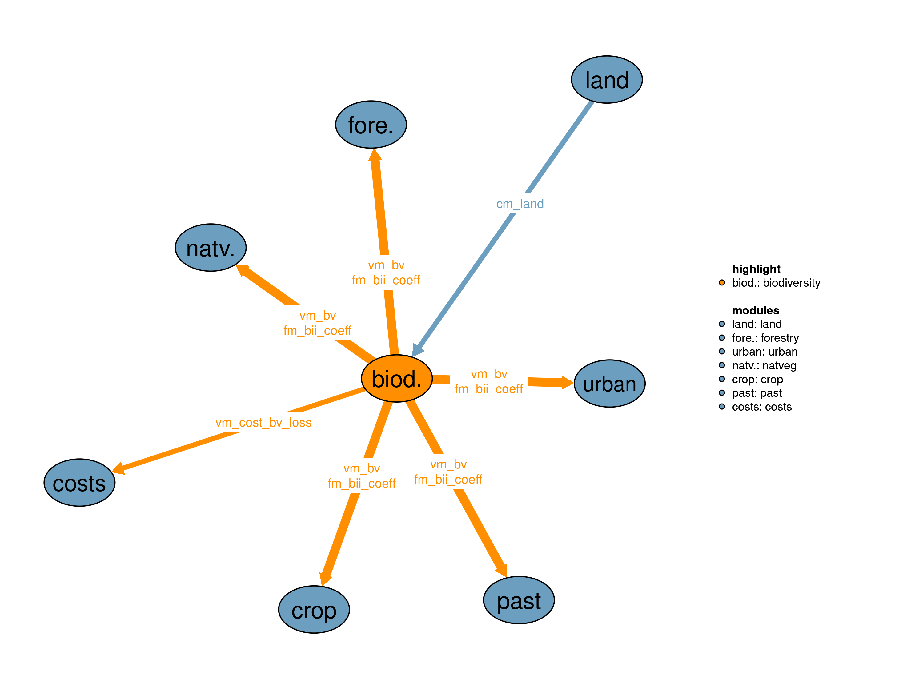
The biodiversity module estimates terrestrial biodiversity stocks for all land types in MAgPIE, based on Biodiversity Intactness Index (BII) coefficients.
| Description | Unit | A | B | |
|---|---|---|---|---|
| pcm_land (j, land) |
Land area in previous time step including possible changes after optimization | \(10^6 ha\) | x |
| Description | Unit | |
|---|---|---|
| fm_bii_coeff (bii_class44, potnatveg) |
Biodiversity Intactness Index coefficients | \(unitless\) |
| vm_bv (j, landcover44, potnatveg) |
Biodiversity stock for all land cover classes | \(Mha\) |
| vm_cost_bv_loss (j) |
Biodiversity cost | \(10^6 USD\) |
In this realisation, the Biodiversity Intactness Index (BII) is calculated separately for each biome type of each biogeographic realm, which results in 71 different spatial units (Olson et al. (2001)). The BII is a relative indicator, wich measures the intactness of local species assemblages (species richness) compared to a reference state (space-for-time approach) (Purvis et al. (2018)). The implementation uses the BII coefficients described in Leclere et al. (2018) and Leclère et al. (2020). The realisation allows to set a lower bound for the BII in the future, based on an annual growth rate.
The Biodiversity Intactness Index (BII) is calculated at the level of 71 biomes.
\[\begin{multline*} v44\_bii(biome44) = \left(\frac{\sum_{j2,potnatveg,landcover44}\left( vm\_bv(j2,landcover44,potnatveg) \cdot f44\_biome(j2,biome44)\right) }{ \sum_{j2,land}\left( pcm\_land(j2,land) \cdot f44\_biome(j2,biome44)\right)}\right) \end{multline*}\]
For each of the 71 biomes, the BII has to meet a minium level based on s44_bii_lower_bound. v44_bii_missing is a technical variable to maintain feasibility in case v44_bii cannot be increased.
\[\begin{multline*} v44\_bii(biome44) + v44\_bii\_missing(biome44) \geq \sum_{ct} p44\_bii\_lower\_bound(ct,biome44) \end{multline*}\]
Costs accrue only for v44_bii_missing. In the best case costs should be zero or close to zero. Costs strongly depend on the choice of s44_bii_lower_bound.
\[\begin{multline*} \sum_{j2} vm\_cost\_bv\_loss(j2) = \sum_{biome44} v44\_bii\_missing(biome44) \cdot s44\_cost\_bii\_missing \end{multline*}\]
Limitations There are no known limitations.
In this realisation, biodiversity stocks are computed for each land cover type by multiplication with Biodiversity Intactness Index (BII) coefficients from the PREDICTS database. The BII is a relative indicator, wich measures the intactness of local species assemblages (species richness) compared to a reference state (space-for-time approach) (Purvis et al. (2018)). In addition, a range-rarity restoration prioritization layer is used in the optimization. This layer is a spatially explicit indicator of the regional relative range-rarity weighted species richness. derived from the IUCN Red List of Threatened Species (IUCN (2020)). It indicates the global importance of a given cell for species conservation, typically of smaller range, as compared to other cells. Conceptually, the range-rarity weighted biodiversity stock is the product of land cover area (Mha), corresponding BII coefficient [0-1] (unitless) and range-rarity layer [0-1] (unitless). The net biodiversity stock loss (resp. gain) of any land-use change decision, weighted by the range-rarity layer, is taxed (resp. subsidized) within the optimization. The implementation uses the methodology described in Leclere et al. (2018) and Leclère et al. (2020).
The net biodiversity stock change is priced.
\[\begin{multline*} vm\_cost\_bv\_loss(j2) = v44\_bv\_loss(j2) \cdot \sum_{ct} p44\_price\_bv\_loss(ct) \end{multline*}\]
Change in biodiversity stock compared to previous time step, divided by time step length.
\[\begin{multline*} v44\_bv\_loss(j2) = \frac{ \left(v44\_bv\_weighted.l(j2) - v44\_bv\_weighted(j2)\right)}{m\_timestep\_length} \end{multline*}\]
Biodiversity stock weighted by range-rarity restoration prioritization layer (f44_rr_layer)
\[\begin{multline*} v44\_bv\_weighted(j2) = f44\_rr\_layer(j2) \cdot \sum_{potnatveg,landcover44} vm\_bv(j2,landcover44,potnatveg) \end{multline*}\]
Limitations The BII indicator has been proposed as a proxy for functional diversity, but here is weighted by an aggegrated conservation priority (range-rarity) layer with no clear linkage to ecosystem functioning outside the priority areas (including areas that stabilise the earth system such as the Amazonas basin or the boreal forest). ‘Biodiversity stocks’ in this realisation are estimated at cluster level, but optimised at the global scale without spatial reference (besides the range-rarity weight). They are therefore theoretically interchangeable across biomes or other spatial units with different biophysical conditions. Scenario design and results based on this realisation should be handled with special caution, in particular when applied in policy contexts. It is strongly advised to complement a positive price on biodiversity loss (resp. gain) in this realization with targeted protection measures (35_natveg).
| Description | Unit | A | B | |
|---|---|---|---|---|
| c44_bii_decrease | Implementation of lower bound for BII | \(binary\) | x | |
| f44_biome (j, biome44) |
Share of biome type in each spatial unit | \(1\) | x | |
| f44_rr_layer (j) |
Range-rarity restoration prioritization layer | \(unitless\) | x | |
| p44_bii_lower_bound (t, biome44) |
Interpolated lower bound for BII over time | \(1\) | x | |
| p44_price_bv_loss (t_all) |
Price (subsidy) for biodiversity stock loss (gain) | \(USD/ha\) | x | |
| p44_start_value (biome44) |
Start value for BII lower bound | \(1\) | x | |
| p44_target_value (biome44) |
Target value for BII lower bound | \(1\) | x | |
| q44_bii (biome44) |
Biodiversity Intactness Index BII | \(1\) | x | |
| q44_bii_target (biome44) |
Missing BII increase for compliance with BII target | \(1\) | x | |
| q44_bv_loss (j) |
Change in biodiversity stock | \(Mha/year\) | x | |
| q44_bv_weighted (j) |
Range-rarity weighted biodiversity stock | \(Mha\) | x | |
| q44_cost | Biodiversity cost | \(10^6 USD\) | x | |
| q44_cost_bv_loss (j) |
Cost of biodiversity loss | \(10^6 USD\) | x | |
| s44_bii_lower_bound | Lower bound for BII | \(1\) | x | |
| s44_cost_bii_missing | Technical costs for missing BII increase | \(USD/unit of BII\) | x | |
| s44_start_price | Price for biodiversity stock loss in start year | \(USD/ha\) | x | |
| s44_start_year | Start year for interpolation towards BII lower bound | \(1\) | x | x |
| s44_target_price | Price for biodiversity stock loss in target year | \(USD/ha\) | x | |
| s44_target_year | Year in which the BII lower bound is reached | \(1\) | x | x |
| v44_bii (biome44) |
Biodiversity Intactness Index BII | \(1\) | x | |
| v44_bii_missing (biome44) |
Missing BII increase for compliance with BII target | \(1\) | x | |
| v44_bv_loss (j) |
Change in biodiversity stock | \(Mha/year\) | x | |
| v44_bv_weighted (j) |
Range-rarity weighted biodiversity stock | \(Mha\) | x |
| description | |
|---|---|
| ac | Age classes |
| ac_to_bii_class_secd(ac, bii_class_secd) | Mapping between forest ageclasses and bii coefficent land cover classes |
| bii_class_secd(bii_class44) | bii coefficent land cover classes secondary vegetation |
| bii_class44 | bii coefficent land cover classes |
| biome44 | biomes |
| ct(t) | Current time period |
| j | number of LPJ cells |
| j2(j) | Spatial Clusters (dynamic set) |
| land | Land pools |
| landcover44 | land cover classes used in bii calculation |
| potnatveg(luh2_side_layers10) | potentially forested biomes |
| t_all(t_ext) | 5-year time periods |
| t(t_all) | Simulated time periods |
| type | GAMS variable attribute used for the output |
Patrick v. Jeetze, Florian Humpenöder
10_land, 11_costs, 30_crop, 31_past, 32_forestry, 34_urban, 35_natveg
IUCN. 2020. “The IUCN Red List of Threatened Species.” 2020. https://www.iucnredlist.org.
Leclère, David, Michael Obersteiner, Mike Barrett, Stuart H. M. Butchart, Abhishek Chaudhary, Adriana De Palma, Fabrice A. J. DeClerck, et al. 2020. “Bending the Curve of Terrestrial Biodiversity Needs an Integrated Strategy.” Nature 585 (7826): 551–56. https://doi.org/10.1038/s41586-020-2705-y.
Leclere, D., M. Obersteiner, R. Alkemade, R. Almond, M. Barrett, G. Bunting, N. Burgess, et al. 2018. “Towards Pathways Bending the Curve Terrestrial Biodiversity Trends Within the 21st Century.” Other. https://doi.org/10.22022/ESM/04-2018.15241.
Olson, David M., Eric Dinerstein, Eric D. Wikramanayake, Neil D. Burgess, George V. N. Powell, Emma C. Underwood, Jennifer A. D’amico, et al. 2001. “Terrestrial Ecoregions of the World: A New Map of Life on Earth: A New Global Map of Terrestrial Ecoregions Provides an Innovative Tool for Conserving Biodiversity.” BioScience 51 (11): 933–38. https://doi.org/10.1641/0006-3568(2001)051[0933:TEOTWA]2.0.CO;2.
Purvis, Andy, Tim Newbold, Adriana De Palma, Sara Contu, Samantha L. L. Hill, Katia Sanchez-Ortiz, Helen R. P. Phillips, et al. 2018. “Chapter Five - Modelling and Projecting the Response of Local Terrestrial Biodiversity Worldwide to Land Use and Related Pressures: The PREDICTS Project.” In Advances in Ecological Research, edited by David A. Bohan, Alex J. Dumbrell, Guy Woodward, and Michelle Jackson, 58:201–41. Next Generation Biomonitoring: Part 1. Academic Press. https://doi.org/10.1016/bs.aecr.2017.12.003.