The urban land module is one of the land modules in MAgPIE (see also the other land modules: 30_crop, 31_past, 32_forestry, 35_natveg). It describes urban settlement areas and estimates their corresponding carbon content and biodiversity values.
| Description | Unit | A | B | |
|---|---|---|---|---|
| fm_bii_coeff (bii_class44, potnatveg) |
Biodiversity Intactness Index coefficients | \(unitless\) | x | x |
| fm_luh2_side_layers (j, luh2_side_layers10) |
luh2 side layers | \(grid cell share\) | x | x |
| pcm_land (j, land) |
Land area in previous time step including possible changes after optimization | \(10^6 ha\) | x | x |
| sm_fix_SSP2 | year until which all parameters are fixed to SSP2 values | \(year\) | x | |
| vm_bv (j, landcover44, potnatveg) |
Biodiversity stock for all land cover classes | \(Mha\) | x | x |
| vm_carbon_stock (j, land, c_pools, stockType) |
Carbon stock in vegetation soil and litter for different land types | \(10^6 tC\) | x | x |
| vm_land (j, land) |
Land area of the different land types | \(10^6 ha\) | x | x |
| Description | Unit | |
|---|---|---|
| vm_cost_urban (j) |
Technical adjustment costs |
Urban Land based on LUH2v2 (Hurtt 2020) cellular (0.5 degree) input dataset, varying with SSP. Cellular level is prescribed via a very high punishment term for deviating from original input values. Regional sums of urban land must add be equal for both model and input data.
Cellular level land is prescribed via a very strong incentive not to deviate from cellular input data. v34_cost1 and v34_cost2 are the cost variables that implement this, for when vm_land(j2,“urban”) is less than and greater than the input data i.e. when reducing or establishing more urban land than in input. This safeguards against infeasible outcomes, where urban land should expand but can not due to NPI or other protected land constraints. In this case it incurs the cost and shifts the land elsewhere in the region.
\[\begin{multline*} v34\_cost1(j2) \geq \sum_{ct}\left( i34\_urban\_area\left(ct, j2\right)\right) - vm\_land(j2,"urban") \end{multline*}\]
\[\begin{multline*} v34\_cost2(j2) \geq vm\_land(j2,"urban") - \sum_{ct}\left( i34\_urban\_area\left(ct, j2\right)\right) \end{multline*}\]
Sum up cost terms with high punishment
\[\begin{multline*} vm\_cost\_urban(j2) = \left(v34\_cost1(j2) + v34\_cost2(j2)\right) \cdot s34\_urban\_deviation\_cost \end{multline*}\]
Regional level urban land must match
\[\begin{multline*} \sum_{cell(i2,j2)} vm\_land(j2,"urban") = \sum_{ct,cell(i2,j2)} i34\_urban\_area(ct,j2) \end{multline*}\]
Biodiversity value (BV)
\[\begin{multline*} vm\_bv\left(j2,"urban", potnatveg\right) = vm\_land(j2,"urban") \cdot fm\_bii\_coeff("urban",potnatveg) \cdot fm\_luh2\_side\_layers(j2,potnatveg) \end{multline*}\]
Limitations Urban land is exogenous and does not interact with other model dynamics, except for reducing available non-urban land pool. Cellular urban land may not exactly match input data due to other land needs in the same cell.
In the static realization, urban land remains static over time with the spatial distribution of 1995 from the LUH2 data set (Hurtt et al. 2018). Carbon stocks are fixed to zero because information on urban land carbon density is missing.
Biodiveristy value (BV)
Limitations Urban land is static over time and corresponding carbon stocks are assumed zero
| Description | Unit | A | B | |
|---|---|---|---|---|
| f34_urbanland (t_all, j, urban_scen34) |
Urban land | x | ||
| i34_urban_area (t_all, j) |
Cellular urban area | x | ||
| q34_bv_urban (j, potnatveg) |
Biodiversity value for urban land | \(Mha\) | x | |
| q34_urban_cell (j) |
Constraint for urban land | x | ||
| q34_urban_cost1 (j) |
Technical punishment equation | x | ||
| q34_urban_cost2 (j) |
Technical punishment equation | x | ||
| q34_urban_land (i) |
Prescribe total regional urban land | x | ||
| s34_urban_deviation_cost | Artificial cost for urban deviation variables | \(USD_{05MER}/ha\) | x | |
| v34_cost1 (j) |
Technical adjustment costs | x | ||
| v34_cost2 (j) |
Technical adjustment costs | x |
| description | |
|---|---|
| ag_pools(c_pools) | Above ground carbon pools |
| bii_class44 | bii coefficent land cover classes |
| c_pools | Carbon pools |
| cell(i, j) | number of LPJ cells per region i |
| ct(t) | Current time period |
| i | all economic regions |
| i2(i) | World regions (dynamic set) |
| j | number of LPJ cells |
| j2(j) | Spatial Clusters (dynamic set) |
| land | Land pools |
| landcover44 | land cover classes used in bii calculation |
| luh2_side_layers10 | side layers from LUH2 |
| potnatveg(luh2_side_layers10) | potentially forested biomes |
| stockType | Carbon stock types |
| t_all(t_ext) | 5-year time periods |
| t(t_all) | Simulated time periods |
| type | GAMS variable attribute used for the output |
| urban_scen34 | Urban scenario |
Jan Philipp Dietrich, Florian Humpenöder, David Meng-Chuen Chen, Benjamin Leon Bodirsky
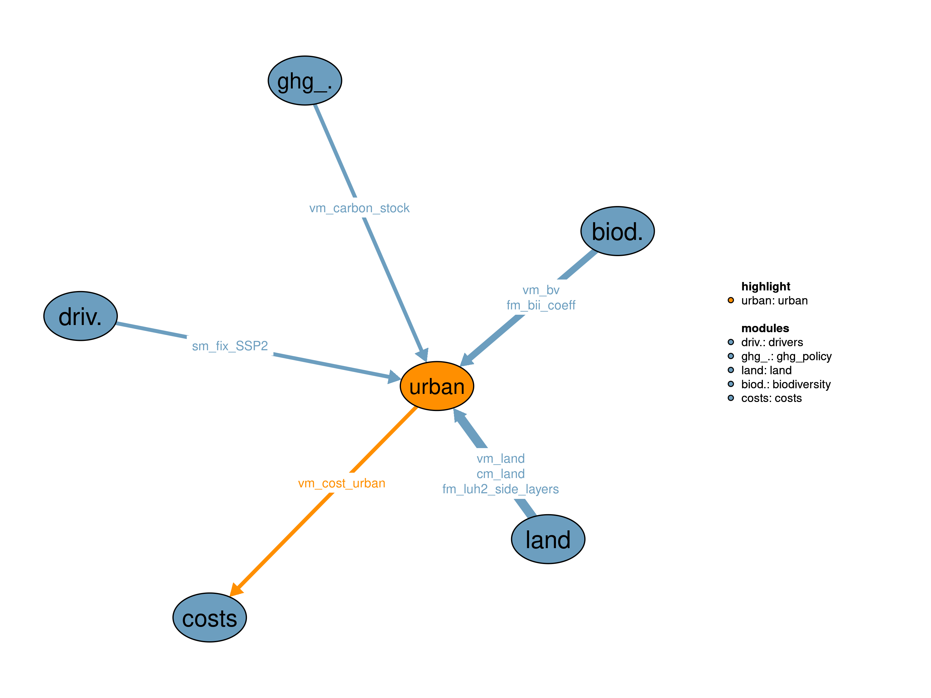
09_drivers, 10_land, 11_costs, 44_biodiversity, 56_ghg_policy
Hurtt, George C, Louise P Chini, Ritvik Sahajpal, Steve E Frolking, Benjamin Bodirsky, Katherine V Calvin, Jonathan C Doelman, et al. 2018. “LUH2: Harmonization of Global Land-Use Scenarios for the Period 850-2100.” AGUFM 2018: GC13A–01.