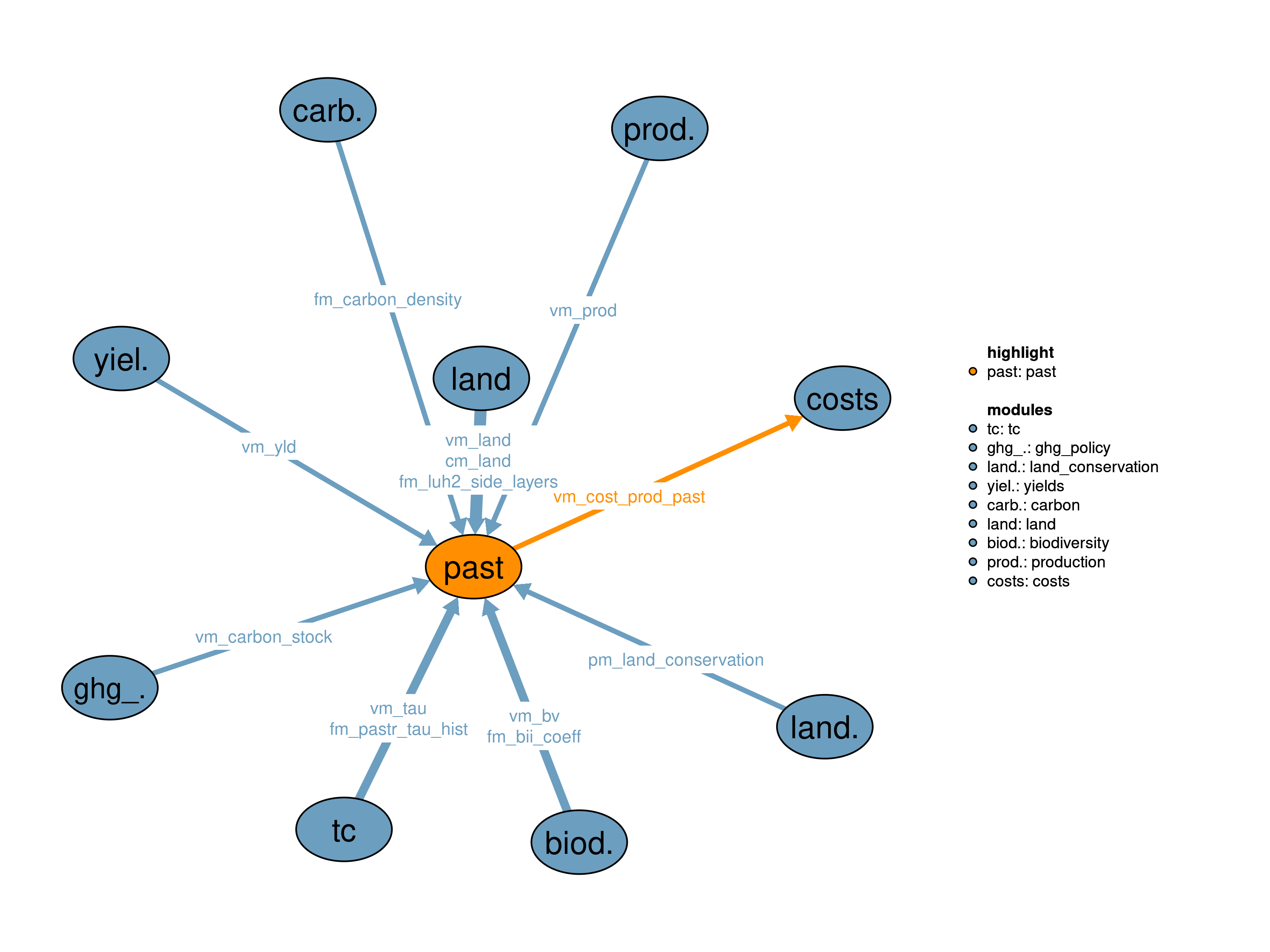
The pasture module determines land used as pasture for livestock rearing. At the same time, it calculates geographically explicit production of pasture biomass and the carbon content of pasture land. Therefore, the module requires cellular information about the carbon density related to the different pasture carbon pools. Furthermore, it delivers regional production costs associated with pastures and biodiversity values for pasture and rangeland.
| Description | Unit | A | B | C | |
|---|---|---|---|---|---|
| fm_bii_coeff (bii_class44, potnatveg) |
Biodiversity Intactness Index coefficients | \(unitless\) | x | x | x |
| fm_carbon_density (t_all, j, land, c_pools) |
LPJmL carbon density for land and carbon pools | \(tC/ha\) | x | x | x |
| fm_luh2_side_layers (j, luh2_side_layers10) |
luh2 side layers | \(grid cell share\) | x | x | x |
| fm_pastr_tau_hist (t_all, h) |
Historical managed pasture tau | \(1\) | x | ||
| pcm_land (j, land) |
Land area in previous time step including possible changes after optimization | \(10^6 ha\) | x | ||
| pm_land_conservation (t, j, land, consv_type) |
Land protection and restoration for all land types | \(10^6 ha\) | x | x | |
| vm_bv (j, landcover44, potnatveg) |
Biodiversity stock for all land cover classes | \(Mha\) | x | x | x |
| vm_carbon_stock (j, land, c_pools, stockType) |
Carbon stock in vegetation soil and litter for different land types | \(10^6 tC\) | x | x | x |
| vm_land (j, land) |
Land area of the different land types | \(10^6 ha\) | x | x | x |
| vm_prod (j, k) |
Production in each cell | \(10^6 tDM/yr\) | x | x | |
| vm_tau (h, tautype) |
Agricultural land use intensity tau | \(1\) | x | ||
| vm_yld (j, kve, w) |
Yields (variable because of technical change) | \(tDM/ha/yr\) | x |
| Description | Unit | |
|---|---|---|
| vm_cost_prod_past (i) |
Costs for putting animals on pastures | \(10^6 USD_{05MER}/yr\) |
In the endo_jun13 realization, pasture area and related carbon stocks are modelled endogenously. The initial spatially explicit patterns of pasture are defined in the module 10_land by the land use input data set. For future time steps, pasture area depends on the demand for biomass from pastures to feed livestock as calculated in the module 70_livestock and from the intensity of pasture utilization (“pasture yield”) as determined in the module 14_yields.
Production of pasture biomass is restricted to pasture area which is delivered as module output together with the resulting geographically explicit production of pasture biomass. Cellular production is calculated by multiplying pasture area vm_land with cellular rainfed pasture yields vm_yld which are delivered by the module 14_yields:
\[\begin{multline*} vm\_prod(j2,"pasture") \leq vm\_land(j2,"past") \cdot vm\_yld(j2,"pasture","rainfed") \end{multline*}\]
On the basis of the required pasture area, cellular above ground carbon stocks are calculated:
\[\begin{multline*} vm\_carbon\_stock(j2,"past",ag\_pools,stockType) = m\_carbon\_stock(vm\_land,fm\_carbon\_density,"past") \end{multline*}\]
In the initial calibration time step, where the pasture calibration factor is calculated that brings pasture biomass demand and pasture area in balance, small costs are attributed to the production of pasture biomass in order to avoid overproduction of pasture in the model:
\[\begin{multline*} vm\_cost\_prod\_past(i2) = \sum_{cell(i2,j2)} vm\_prod(j2,"pasture") \cdot s31\_fac\_req\_past \end{multline*}\]
For all following time steps, factor requriements s31_fac_req_past are set to zero. By estimating the different area of managed pasture and rangeland via the luh2 side layers, the biodiversity value for pastures and rangeland is calculated in following:
\[\begin{multline*} vm\_bv(j2,"manpast",potnatveg) = vm\_land(j2,"past") \cdot fm\_luh2\_side\_layers(j2,"manpast") \cdot fm\_bii\_coeff("manpast",potnatveg) \cdot fm\_luh2\_side\_layers(j2,potnatveg) \end{multline*}\]
\[\begin{multline*} vm\_bv(j2,"rangeland",potnatveg) = vm\_land(j2,"past") \cdot fm\_luh2\_side\_layers(j2,"rangeland") \cdot fm\_bii\_coeff("rangeland",potnatveg) \cdot fm\_luh2\_side\_layers(j2,potnatveg) \end{multline*}\]
Total grassland area cannot be smaller than legally protected grassland area
Limitations No consideration of generic differences between extensive and intensive grazing systems, of explicit pasture management options and of related degradation of pastures.
In the grasslands_apr22 realization, grassland areas and related carbon stocks are modelled endogenously. The initial spatially explicit patterns of grasslands (“past”) are defined in the module 10_land by the land use input data set. These areas are further divided into rangelands and managed pastures under different management assumptions. For future time steps, grasslands spatial distribution depend on the demand of grass biomass to feed livestock as calculated in the module 70_livestock and from the intensity of grassland utilization (“grassland yields”). Grassland yields are defined separately for rangelands and managed pasture based on historical estimates or areas and biomass production for these two systems. Managed pastures yields can be increased endogenously by investments in technology as calculated in 13_tc. Rising yields alter the nitrogen budged on grasslands triggering costs for N inorganic fertilization as calculated in 50_nr_soil_budget and control the balance between intensive and extensive grass biomass production.
Grassland production is estimated by multiplying grassland areas and yields. Technological change is applied to managed pastures yields through ‘vm_tau’, whereas rangeland yields are kept unaltered after the preloop calibration of ‘i31_grass_yields’.
\[\begin{multline*} vm\_prod(j2,"pasture") \leq v31\_grass\_area(j2,"range") \cdot \sum_{ct}i31\_grass\_yields(ct,j2,"range") + v31\_grass\_area(j2,"pastr") \cdot \sum_{ct}i31\_grass\_yields(ct,j2,"pastr") \cdot \sum_{cell(i2,j2), supreg(h2,i2)}\left(\frac{ vm\_tau\left(h2, "pastr"\right) }{ fm\_pastr\_tau\_hist("y1995",h2)}\right) \end{multline*}\]
The sum of managed pastures and rangelands areas equal the parent land class pastures areas in ‘vm_land’.
\[\begin{multline*} vm\_land(j2,"past") = \sum_{grassland} v31\_grass\_area(j2,grassland) \end{multline*}\]
To avoid unrealistic conversions between rangelands and managed pastures areas, a cost is associated with the expansion of rangelands and managed pastures ‘v31_cost_grass_expansion’ in comparison with areas in the previous time step ‘pc31_grass’.
\[\begin{multline*} v31\_cost\_grass\_expansion\left(j2, grassland\right) \geq \left(v31\_grass\_area\left(j2, grassland\right) - pc31\_grass(j2,grassland)\right) \cdot s31\_cost\_expansion \end{multline*}\]
Cost of production account for the cost of moving animals to grassland areas plus the costs of expanding aras of production.
\[\begin{multline*} vm\_cost\_prod\_past(i2) = \sum_{cell(i2,j2)} vm\_prod(j2,"pasture") \cdot s31\_cost\_grass\_prod + \sum_{cell(i2,j2), grassland} v31\_cost\_grass\_expansion(j2,grassland) \end{multline*}\]
On the basis of the required pasture area, cellular above ground carbon stocks are calculated:
\[\begin{multline*} vm\_carbon\_stock(j2,"past",ag\_pools,stockType) = m\_carbon\_stock(vm\_land,fm\_carbon\_density,"past") \end{multline*}\]
By estimating the different area of managed pasture and rangeland via the luh2 side layers, the biodiversity value for pastures and rangeland is calculated in following:
\[\begin{multline*} vm\_bv(j2,"manpast",potnatveg) = vm\_land(j2,"past") \cdot fm\_luh2\_side\_layers(j2,"manpast") \cdot fm\_bii\_coeff("manpast",potnatveg) \cdot fm\_luh2\_side\_layers(j2,potnatveg) \end{multline*}\]
\[\begin{multline*} vm\_bv(j2,"rangeland",potnatveg) = vm\_land(j2,"past") \cdot fm\_luh2\_side\_layers(j2,"rangeland") \cdot fm\_bii\_coeff("rangeland",potnatveg) \cdot fm\_luh2\_side\_layers(j2,potnatveg) \end{multline*}\]
Grassland yields for rangelands and managed pastures are calibrated to match estimated historical pasture productivity. The following equations calibrate the grassland cellular yield patterns (‘f31_grassl_yld’) to match ‘estimated historical yields’ (‘i31_grass_hist_yld’) by calculating a calibration term called ‘i31_grass_calib’. For most cases, ‘i31_grass_calib’ is the ratio of the ‘i31_grass_hist_yld’ and modeled yields (‘i31_grass_modeled_yld’) given historic grassland area patterns (‘i31_grassl_areas’) and cellular yields coming from crop models like LPJmL ‘f31_grassl_yld’. In these cases, ‘i31_grass_calib’ represents a purely relative calibration factor that depends only on the initial conditions of the starting year.
However, when estimated yields ‘i31_grass_hist_yld’ are significantly higher than given by the cellular yield inputs ‘f31_grassl_yld’ we refer to this as an underestimated baseline. In this situation the relative calibration terms can lead to unrealistically large yields in the case of future yield increases within the cellular yield patterns.
To address this issue, we introduce the factor ‘i31_lambda_grass’ that determines the degree to which the baseline ‘i31_grass_hist_yld’ is under- or overestimated by the modeled yields ‘i31_grass_modeled_yld’. This factor is used to control whether the calibration factor is applied as an absolute or relative change. For ‘i31_grass_hist_yld’ smaller than ‘i31_grass_modeled_yld’ (overestimated baseline) ‘i31_lambda_grass’ is 1, which is equivalent to an entirely relative calibration. For underestimated yields, ‘i31_lambda_grass’ is calculated as the squared root of the ratio between modeled yields ‘i31_grass_modeled_yld’ and the historical estimates ‘i31_grass_hist_yld’. For underestimated yields, as ‘i31_lambda_grass’ approaches 0, it reduces the applied relative change resulting in a mean change increasingly similar to an additive term (Heinke et al. (2013)). This concept is referred to as limited calibration, as it limits the calibration to an additive term in case of a strongly underestimated baseline. The scalar
i31_grass_yields(t,j,grassland) = f31_grassl_yld(t,j,grassland,"rainfed");
i31_grassl_areas(t_all,j) =  sum(grassland, f31_LUH2v2(t_all,j,grassland));
i31_grass_hist_yld(t_past,i,grassland) = (f31_grass_bio(t_past,i, grassland) /
                sum(cell(i,j),f31_LUH2v2(t_past,j,grassland)))$(sum(cell(i,j), f31_LUH2v2(t_past,j,grassland))>0);
i31_grass_modeled_yld(t_past,i,grassland)
   = (sum(cell(i,j),i31_grass_yields(t_past,j,grassland) * f31_LUH2v2(t_past,j,grassland)) /
      sum(cell(i,j),f31_LUH2v2(t_past,j,grassland)))$(sum(cell(i,j), f31_LUH2v2(t_past,j,grassland))>0)
   + (sum(cell(i,j),i31_grassl_areas(t_past,j) * i31_grass_yields(t_past,j,grassland)) /
      sum(cell(i,j),i31_grassl_areas(t_past,j)))$(sum(cell(i,j), f31_LUH2v2(t_past,j,grassland))=0);
loop(t,
     if(sum(sameas(t,"y1995"),1)=1,
          if    ((s31_limit_calib = 0),
               i31_lambda_grass(t,i,grassland) = 1;
          Elseif (s31_limit_calib =1 ),
               i31_lambda_grass(t,i,grassland) =
                    1$(i31_grass_hist_yld(t,i,grassland) <= i31_grass_modeled_yld(t,i,grassland))
                    + sqrt(i31_grass_modeled_yld(t,i,grassland)/i31_grass_hist_yld(t,i,grassland))$
                    (i31_grass_hist_yld(t,i,grassland) > i31_grass_modeled_yld(t,i,grassland));
          );
          i31_grassl_yld_hist_reg(t,i,grassland) = i31_grass_hist_yld(t,i,grassland);
     Else
          i31_grass_modeled_yld(t,i,grassland) = i31_grass_modeled_yld(t-1,i,grassland);
          i31_grassl_yld_hist_reg(t,i,grassland)  = i31_grassl_yld_hist_reg(t-1,i,grassland);
          i31_lambda_grass(t,i,grassland)   = i31_lambda_grass(t-1,i,grassland);
     );
);
The calibrated cellular yield ‘i31_grass_yields’ is calculated for each time step depending on the constant values ‘i31_grass_modeled_yld’, ‘i31_grassl_yld_hist_reg’, ‘i31_lambda_grass’ and the uncalibrated, cellular yield ‘f31_grassl_yld’ following the idea of eq. (9) in Heinke et al. (2013):
i31_grass_calib(t,j,grassland) =
  1 + (sum(cell(i,j), i31_grassl_yld_hist_reg(t,i,grassland) - i31_grass_modeled_yld(t,i,grassland)) /
                             f31_grassl_yld(t,j,grassland,"rainfed") *
      (f31_grassl_yld(t,j,grassland,"rainfed") / (sum(cell(i,j),i31_grass_modeled_yld(t,i,grassland))+10**(-8))) **
                             sum(cell(i,j),i31_lambda_grass(t,i,grassland)))$(f31_grassl_yld(t,j,grassland,"rainfed")>0);
i31_grass_yields(t,j,"range") = i31_grass_yields(t,j,"range") * i31_grass_calib(t,j,"range");
i31_grass_yields(t,j,"pastr") = i31_grass_yields(t,j,"pastr") * i31_grass_calib(t,j,"pastr");
Note that the calculation is split into two parts for better readability.
Socioeconomic and environmental conditions determine the potential managed pastures areas (‘i31_manpast_suit’). ‘i31_manpast_suit’ is estimated by determining areas with more than five inhabitants per km2 and with aridity greater than 0.5 following the methodology established by Klein Goldewijk et al. (2017)
v31_grass_area.up(j,"pastr") = i31_manpast_suit(t,j);Total grassland area cannot be smaller than legally protected grassland area
vm_land.lo(j,"past") = sum(consv_type, pm_land_conservation(t,j,"past",consv_type));Limitations We currently do not accout for specific differences within intensive pasture management systems and related degradation of grasslands for both rangelands or managed pastures. Grass production costs and conversion costs between grassland types are set 1 USD05MER per unit due to lack of data.
In the static realization, pasture areas are constant over time, independent from developments in the livestock sector and land competition.
Pasture areas are fixed to the initial spatially explicit patterns defined in the module 10_land by the land use input data set.
vm_land.fx(j,"past") = pcm_land(j,"past");Correspondingly, also the above ground carbon stocks related to pasture areas are fixed.
vm_carbon_stock.fx(j,"past",ag_pools) =
          pcm_land(j,"past")*fm_carbon_density(t,j,"past",ag_pools);
Also the biodiversity value (BV) for pasture is fixed
vm_bv.fx(j,"manpast",potnatveg) =
                    pcm_land(j,"past") * fm_luh2_side_layers(j,"manpast") * fm_bii_coeff("manpast",potnatveg) * fm_luh2_side_layers(j,potnatveg);
vm_bv.fx(j,"rangeland",potnatveg) =
                    pcm_land(j,"past") * fm_luh2_side_layers(j,"rangeland") * fm_bii_coeff("rangeland",potnatveg) * fm_luh2_side_layers(j,potnatveg);
Regional costs associated with pasture management are set to zero.
vm_cost_prod_past.fx(i) = 0;Limitations There are no computational limitations to this realization. Since pasture areas are static, they do not respond to demand trajectories and trends in the land use and agricultural sectors like intensification pathways, increasing production of animal products, bioenergy production or afforestation policies. This may lead to an inconsistent overall picture of future land use dynamics.
| Description | Unit | A | B | C | |
|---|---|---|---|---|---|
| f31_grass_bio (t_all, i, grassland) |
Estimated regional grass biomass consumption in the past | \(tDM\) | x | ||
| f31_grassl_yld (t_all, j, grassland, w) |
LPJmL potential yields per cell (rainfed only) | \(tDM/ha\) | x | ||
| f31_LUH2v2 (t_all, j, f31_luh) |
Different land type areas | \(10^6 ha\) | x | ||
| f31_pastr_suitability (t_all, j, ssp_past) |
Areas suitable for pasture management | \(10^6 ha\) | x | ||
| i31_grass_calib (t_all, j, grassland) |
Regional grassland calibration factor correcting for FAO yield levels | \(1\) | x | ||
| i31_grass_hist_yld (t_all, i, grassland) |
FAO gassland yields | \(tDM/ha\) | x | ||
| i31_grass_modeled_yld (t_all, i, grassland) |
Biophysical input yields average over region and grassland cover type at the historical reference year | \(tDM/ha\) | x | ||
| i31_grass_yields (t_all, j, grassland) |
Cellular biophysical input yields | \(tDM/ha\) | x | ||
| i31_grassl_areas (t_all, j) |
Celullar grassland areas | \(10^6 ha\) | x | ||
| i31_grassl_yld_hist_reg (t, i, grassland) |
Grassland FAO yields per region at the historical referende year | \(tDM/ha\) | x | ||
| i31_lambda_grass (t, i, grassland) |
Grassland Scaling factor for non-linear management calibration | \(1\) | x | ||
| i31_manpast_suit (t_all, j) |
Areas suitable for managed pastures | \(10^6 ha\) | x | ||
| pc31_grass (j, grassland) |
Grassland areas in previous time step | \(10^6 ha\) | x | ||
| q31_bv_manpast (j, potnatveg) |
Biodiversity value for managed pastures | \(Mha\) | x | x | |
| q31_bv_rangeland (j, potnatveg) |
Biodiversity value for rangeland | \(Mha\) | x | x | |
| q31_carbon (j, ag_pools, stockType) |
Above ground carbon content calculation for pasture | \(10^6 tC\) | x | x | |
| q31_cost_prod_past (i) |
Costs for putting animals on pastures | \(10^6 USD_{05MER}/yr\) | x | x | |
| q31_expansion_cost (j, grassland) |
Grassland expansion cost constraint | \(10^6 USD_{05MER}\) | x | ||
| q31_pasture_areas (j) |
Total grassland calculation | \(10^6 ha\) | x | ||
| q31_prod (j) |
Cellular pasture production constraint | \(10^6 tDM/yr\) | x | ||
| q31_prod_pm (j) |
Cellular grass production constraint | \(10^6 tDM/yr\) | x | ||
| s31_cost_expansion | Grasslands expansion costs | \(USD_{05MER}/hectare\) | x | ||
| s31_cost_grass_prod | Grasslands factor costs | \(USD_{05MER}/tDM\) | x | ||
| s31_fac_req_past | Factor requirements | \(USD_{05MER}/tDM\) | x | ||
| s31_limit_calib | Relative managament calibration switch | \(1=limited 0=pure relative\) | x | ||
| v31_cost_grass_expansion (j, grassland) |
Costs of grassland expansion | \(10^6 USD_{05MER}\) | x | ||
| v31_grass_area (j, grassland) |
Grassland areas | \(10^6 ha\) | x |
| description | |
|---|---|
| ag_pools(c_pools) | Above ground carbon pools |
| bii_class44 | bii coefficent land cover classes |
| c_pools | Carbon pools |
| cell(i, j) | number of LPJ cells per region i |
| consv_type | Type of land conservation |
| ct(t) | Current time period |
| f31_luh | LHUv2 land cover types |
| grass_from31(grassland) | pasture management options |
| grass_to31(grassland) | pasture management options |
| grassland(f31_luh) | Grassland cover types (pastr = managed pastures and range = rangelands) |
| h | all superregional economic regions |
| h2(h) | Superregional (dynamic set) |
| i | all economic regions |
| i2(i) | World regions (dynamic set) |
| j | number of LPJ cells |
| j2(j) | Spatial Clusters (dynamic set) |
| k(kall) | Primary products |
| kve(k) | Land-use activities |
| land | Land pools |
| landcover44 | land cover classes used in bii calculation |
| luh2_side_layers10 | side layers from LUH2 |
| potnatveg(luh2_side_layers10) | potentially forested biomes |
| ssp_past | SSP scenarios for pasture suitability areas |
| stockType | Carbon stock types |
| supreg(h, i) | mapping of superregions to its regions |
| t_all(t_ext) | 5-year time periods |
| t_past(t_all) | Timesteps with observed data |
| t(t_all) | Simulated time periods |
| tautype | tc type |
| type | GAMS variable attribute used for the output |
| w | Water supply type |
Isabelle Weindl, Jan Philipp Dietrich, Marcos Alves
10_land, 11_costs, 13_tc, 14_yields, 17_production, 22_land_conservation, 44_biodiversity, 52_carbon, 56_ghg_policy
Heinke, J., S. Ostberg, S. Schaphoff, K. Frieler, C. Müller, D. Gerten, M. Meinshausen, and W. Lucht. 2013. “A New Climate Dataset for Systematic Assessments of Climate Change Impacts as a Function of Global Warming.” Geoscientific Model Development 6 (5): 1689–1703. https://doi.org/10.5194/gmd-6-1689-2013.
Klein Goldewijk, Kees, Arthur Beusen, Jonathan Doelman, and Elke Stehfest. 2017. “Anthropogenic Land Use Estimates for the Holocene – Hyde 3.2.” Earth System Science Data 9 (2): 927–53. https://doi.org/10.5194/essd-9-927-2017.