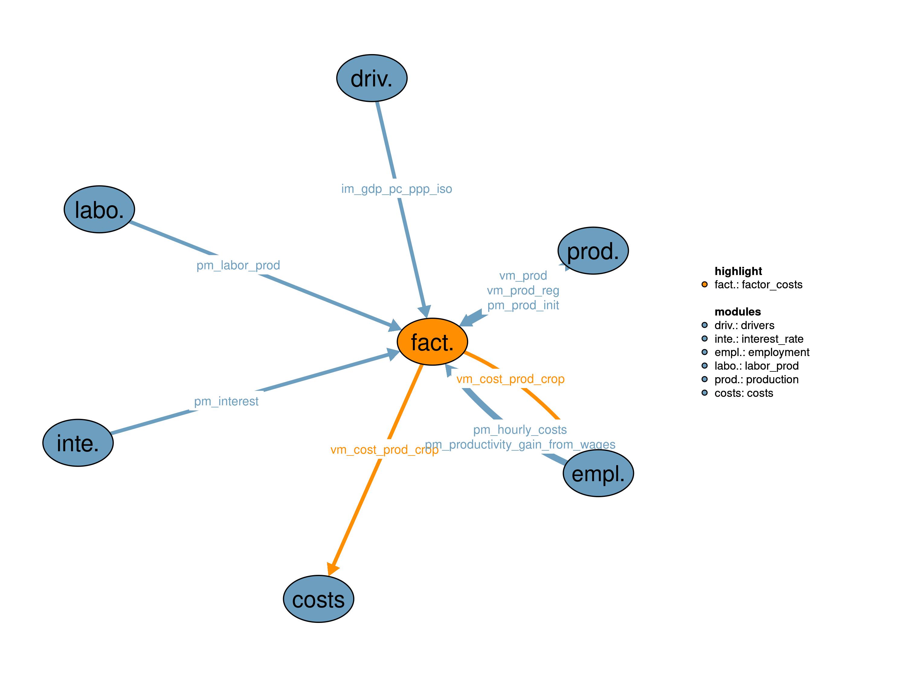
This module is used to calculate factor costs of production in crop activities. The costs of factors of production included in this module are specifically of labor, capital, and energy and related costs. The costs are crop-specific, and pass to the the cost function in 11_costs. Thus, factor costs will contribute to and influence the choice of production pattern in the model.
| Description | Unit | A | B | C | |
|---|---|---|---|---|---|
| im_gdp_pc_ppp_iso (t_all, iso) |
Per capita income in purchasing power parity | \(USD_{05PPP}/cap/yr\) | x | x | x |
| pm_hourly_costs (t, i, wage_scen) |
Hourly labor costs in agriculture on regional level before and after including wage scenario | \(USD_{MER}05/hour\) | x | x | x |
| pm_interest (t_all, i) |
Interest rate in each region and timestep | \(\%/yr\) | x | x | |
| pm_labor_prod (t, j) |
labor productivity factor | \(1\) | x | x | x |
| pm_prod_init (j, kcr) |
Production initialization for year 1995 | \(tDM/yr\) | x | x | |
| pm_productivity_gain_from_wages (t, i) |
Multiplicative factor describing productivity gain related to higher wages | \(1\) | x | x | x |
| vm_prod (j, k) |
Production in each cell | \(10^6 tDM/yr\) | x | x | |
| vm_prod_reg (i, kall) |
Regional aggregated production | \(10^6 tDM/yr\) | x | x |
| Description | Unit | |
|---|---|---|
| vm_cost_prod_crop (i, req) |
Regional factor costs of capital and labor for crop production | \(10^6 USD_{05MER}/yr\) |
This realization relates factor costs to volume of production of a given crop. The latter 17_production depends on area harvested from 30_crop and yields from 14_yields. In other words, in this implementation, factor costs entirely depend on the volume of production. As such, there are no incentives to allocate and concentrate production into more productive cells.
\[\begin{multline*} vm\_cost\_prod\_crop(i2,"labor") = \sum_{kcr}\left( vm\_prod\_reg(i2,kcr) \cdot \sum_{ct}i38\_fac\_req(ct,i2,kcr)\right) \cdot \sum_{ct}\left(p38\_cost\_share(ct,i2,"labor") \cdot \left(\frac{1}{pm\_productivity\_gain\_from\_wages(ct,i2)}\right) \cdot \left(\frac{pm\_hourly\_costs(ct,i2,"scenario") }{ pm\_hourly\_costs(ct,i2,"baseline")}\right)\right) \end{multline*}\]
\[\begin{multline*} vm\_cost\_prod\_crop(i2,"capital") = \sum_{kcr}\left( vm\_prod\_reg(i2,kcr) \cdot \sum_{ct}i38\_fac\_req(ct,i2,kcr)\right) \cdot \sum_{ct}p38\_cost\_share(ct,i2,"capital") \end{multline*}\]
The factor costs for crops vm_cost_prod_crop are calculated as product of production quantity vm_prod_reg and crop-specific factor requirements (either global or regional averages) per volume of production i38_fac_req. The volume depending factor requirements, which remain fixed overtime, are obtained from FAO Value of Production, to which the USDA factor cost share out of total costs was applied. Labor and capital costs are split by applying the corresponding share out of total factor costs. To account for increased hourly labor costs and producitivity in case of an external wage scenario, the total labor costs are scaled by the corresponding increase in hourly labor costs and the related productivity gain from 36_employment.
It is worth to mention again that the factor costs in this module do not include land rents (as MAgPIE calculates land rents endogenously), chemical fertilizer costs (as they are calculated in 50_nr_soil_budget module), and costs of agricultural intermediate inputs such as seeds (to avoid double counting in the model).
Limitations This realization assumes that factor costs, within a region, purely depend on the production and are independent of the area under cultivation. By implication, cases in which the harvested area could significantly influence factors costs are hardly accounted in this realization.
The main goal of this realization is to improve crop patterns at different spatial scales. Specifically, the goal is reached by reducing capital relocation flexibility between crop types. In the “sticky” realization, the factor costs are separated into variable and capital investment costs. Then, capital is furtherly divided into immobile and mobile, where mobility is defined between crops. In this way, changes in cropland are favored in locations with existing capital stocks.
Labor costs: The labor costs are calculated by multiplying regional aggregated production with labor requirments per output. To account for increased hourly labor costs and producitivity in case of an external wage scenario, the total labor costs are scaled by the corresponding increase in hourly labor costs and the related productivity gain from 36_employment.
\[\begin{multline*} vm\_cost\_prod\_crop(i2,"labor") = \sum_{kcr}\left(vm\_prod\_reg(i2,kcr) \cdot \sum_{ct}\left(p38\_labor\_need(ct,i2,kcr) \cdot \left(\frac{1}{pm\_productivity\_gain\_from\_wages(ct,i2)}\right) \cdot \left(\frac{pm\_hourly\_costs(ct,i2,"scenario") }{ pm\_hourly\_costs(ct,i2,"baseline")}\right)\right)\right) \end{multline*}\]
Investment costs: Investment are the summation of investment in mobile and immobile capital. The costs are annuitized, and corrected to make sure that the annual depreciation of the current time-step is accounted for.
\[\begin{multline*} vm\_cost\_prod\_crop(i2,"capital") = \left(\sum_{cell(i2,j2),kcr}v38\_investment\_immobile(j2,kcr) +\sum_{cell(i2,j2)}v38\_investment\_mobile(j2)\right) \cdot \left(\left(1-s38\_depreciation\_rate\right) \cdot \sum_{ct}\left(\frac{pm\_interest(ct,i2)}{\left(1+pm\_interest(ct,i2)\right)}\right) + s38\_depreciation\_rate\right) \end{multline*}\]
Each cropping activity requires a certain capital stock that depends on the production. The following equations make sure that new land expansion is equipped with capital stock, and that depreciation of pre-existing capital is replaced. Since the mobility of capital is defined over crop-type, immobile capital is set over specific crop types and locations.
\[\begin{multline*} v38\_investment\_immobile(j2,kcr) \geq vm\_prod(j2,kcr) \cdot \sum_{cell(i2,j2)}\left(\sum_{ct}p38\_capital\_need(ct,i2,kcr,"immobile")\right)- \sum_{ct}p38\_capital\_immobile(ct,j2,kcr) \end{multline*}\]
On the other hand, the mobile capital is needed by all crop activities in each location, so it is defined over each j2 cell.
\[\begin{multline*} v38\_investment\_mobile(j2) \geq \sum_{cell(i2,j2),kcr}\left(vm\_prod(j2,kcr) \cdot \sum_{ct}p38\_capital\_need(ct,i2,kcr,"mobile")\right)- \sum_{ct}p38\_capital\_mobile(ct,j2) \end{multline*}\]
Estimate capital stock based on capital remuneration. We assume that in 1994 and 1995 production is the same and the stocks gets depreciated from 1994. Update of existing stocks
Capital update from the last investment
Limitations This realization assumes that factor costs, within a region, purely depend on the production and are independent of the area under cultivation. By implication, cases in which the harvested area could significantly influence factors costs are hardly accounted in this realization.
This realization is based on sticky_feb18, but in addition includes a CES production function, which accounts for climate change impacts on labor productivity provided by 37_labor_prod, and wage increase impact on labor productivity based on wages in 36_employment. The main goal of this realization is to improve crop patterns at different spatial scales. Specifically, the goal is reached by reducing capital relocation flexibility between crop types. In the “sticky” realization, the factor costs are separated into variable labor cost and capital investment cost. Then, capital is further divided into immobile and mobile, where mobility is defined between crops. In this way, changes in cropland are favored in locations with existing capital stocks.
Constant elasticity of substitution (CES) production function for one unit of output. The CES function accounts for capital v38_capital_need and labor v38_laborhours_need requirements. The efficiency of labor is affected by the labor productivity factor pm_labor_prod based on climate change impacts, which is provided by the labor productivity module 37_labor_prod, and by the factor pm_productivity_gain_from_wages based on increased wages from 36_employment. The calculation of total capital and labor costs is covered by the equations q38_cost_prod_crop and q38_cost_prod_inv. The conceptual and analytical details of the CES function including the labor productivity factor are documented in Orlov and Humpenöder (2021).
\[\begin{multline*} i38\_ces\_scale(j2,kcr) \cdot \left(i38\_ces\_shr(j2,kcr) \cdot \sum_{mobil38} v38\_capital\_need(j2,kcr,mobil38)^{\left(-s38\_ces\_elast\_par\right) }+ \left(1 - i38\_ces\_shr(j2,kcr)\right) \cdot \left(\sum_{ct}\left( pm\_labor\_prod(ct,j2) \cdot \sum_{cell(i2,j2)} pm\_productivity\_gain\_from\_wages(ct,i2)\right) \cdot v38\_laborhours\_need(j2,kcr)\right)^{\left(-s38\_ces\_elast\_par\right)}\right)^{\left(-\frac{1}{s38\_ces\_elast\_par}\right) } = 1 \end{multline*}\]
Labor costs: The labor costs are calculated by multiplying regional aggregated production with labor requirements (in hours) per output unit and wages from 36_employment.
\[\begin{multline*} vm\_cost\_prod\_crop(i2,"labor") = \sum_{kcr}\left(\sum_{cell(i2,j2)}\left( vm\_prod(j2,kcr) \cdot v38\_laborhours\_need(j2,kcr) \cdot \sum\left(ct, pm\_hourly\_costs(ct,i2,"scenario")\right)\right)\right) \end{multline*}\]
Investment costs: Investment are the summation of investment in mobile and immobile capital. The costs are annuitized, and corrected to make sure that the annual depreciation of the current time-step is accounted for.
\[\begin{multline*} vm\_cost\_prod\_crop(i2,"capital") = \left(\sum_{cell(i2,j2),kcr}v38\_investment\_immobile(j2,kcr) +\sum_{cell(i2,j2)}v38\_investment\_mobile(j2)\right) \cdot \left(\left(1-s38\_depreciation\_rate\right) \cdot \sum_{ct}\left(\frac{pm\_interest(ct,i2)}{\left(1+pm\_interest(ct,i2)\right)}\right) + s38\_depreciation\_rate\right) \end{multline*}\]
Each cropping activity requires a certain capital stock that depends on the production. The following equations make sure that new land expansion is equipped with capital stock, and that depreciation of pre-existing capital is replaced. Since the mobility of capital is defined over crop-type, immobile capital is set over specific crop types and locations.
\[\begin{multline*} v38\_investment\_immobile(j2,kcr) \geq vm\_prod(j2,kcr) \cdot v38\_capital\_need(j2,kcr,"immobile") - \sum_{ct} p38\_capital\_immobile(ct,j2,kcr) \end{multline*}\]
On the other hand, the mobile capital is needed by all crop activities in each location, so it is defined over each j2 cell.
\[\begin{multline*} v38\_investment\_mobile(j2) \geq \sum_{kcr}\left( vm\_prod(j2,kcr) \cdot v38\_capital\_need(j2,kcr,"mobile")\right) - \sum_{ct} p38\_capital\_mobile(ct,j2) \end{multline*}\]
Estimate capital stock based on capital remuneration. We assume that in 1994 and 1995 production is the same and the stocks gets depreciated from 1994. Update of existing stocks
Capital update from the last investment
Limitations This realization assumes that factor costs, within a region, purely depend on the production and are independent of the area under cultivation. By implication, cases in which the harvested area could significantly influence factors costs are hardly accounted in this realization.
| Description | Unit | A | B | C | |
|---|---|---|---|---|---|
| f38_fac_req (kcr) |
Factor requirement costs in 2005 | \(USD_{05MER}/tDM\) | x | x | x |
| f38_fac_req_fao_reg (t_all, i, kcr) |
Factor requirement costs | \(USD_{05MER}/tDM\) | x | x | x |
| f38_historical_share (t_all, i) |
Historical capital share | x | x | x | |
| f38_reg_parameters (reg) |
Parameters for regression | x | x | x | |
| i38_ces_scale (j, kcr) |
Scaling factor for total factor productivity | \(1\) | x | ||
| i38_ces_shr (j, kcr) |
Share parameter for CES function | \(1\) | x | ||
| i38_fac_req (t_all, i, kcr) |
Factor requirements | \(USD_{05MER}/tDM\) | x | x | x |
| p38_capital_immobile (t, j, kcr) |
Preexisting immobile capital stocks before investment | \(10^6 USD_{05MER}\) | x | x | |
| p38_capital_mobile (t, j) |
Preexisting mobile capital stocks before investment | \(10^6 USD_{05MER}\) | x | x | |
| p38_capital_need (t, i, kcr, mobil38) |
Capital requirements per unit of output | \(USD_{05MER}/ton DM\) | x | x | |
| p38_cost_share (t, i, req) |
Capital and labor shares of the regional factor costs for crop production | \(1\) | x | x | x |
| p38_croparea_start (j, w, kcr) |
Agricultural land initialization area | \(10^6 ha\) | x | x | |
| p38_intr_depr (t, i) |
Factor from interest and depreciation rate | \(1\) | x | ||
| p38_labor_need (t, i, kcr) |
Labor input costs per unit of output | \(USD_{05MER}/ton DM\) | x | x | |
| p38_share_calibration (i) |
Summation factor used to calibrate calculated capital shares with historical values | \(1\) | x | x | x |
| q38_ces_prodfun (j, kcr) |
CES production function for one unit of output | \(1\) | x | ||
| q38_cost_prod_capital (i) |
Regional capital input costs for crop production | \(10^6 USD_{05MER}\) | x | x | |
| q38_cost_prod_crop_capital (i) |
Regional capital costs for crop production | \(10^6 USD_{05MER}/yr\) | x | ||
| q38_cost_prod_crop_labor (i) |
Regional labor costs for crop production | \(10^6 USD_{05MER}/yr\) | x | ||
| q38_cost_prod_labor (i) |
Regional labor input costs for crop production | \(10^6 USD_{05MER}\) | x | x | |
| q38_investment_immobile (j, kcr) |
Cellular immobile investments into farm capital | \(10^6 USD_{05MER}\) | x | x | |
| q38_investment_mobile (j) |
Cellular mobile investments into farm capital | \(10^6 USD_{05MER}\) | x | x | |
| s38_ces_elast_par | Elasticity parameter for CES function | \(1\) | x | ||
| s38_ces_elast_subst | Elasticity of substitution in CES function | \(1\) | x | ||
| s38_depreciation_rate | depreciation rate | \(share of costs\) | x | x | |
| s38_fix_capital_need | Year until which capital requirements are fixed | x | |||
| s38_immobile | immobile capital | \(share\) | x | x | |
| v38_capital_need (j, kcr, mobil38) |
Captial required per unit of output | \(USD_{05MER}/ton DM\) | x | ||
| v38_investment_immobile (j, kcr) |
Investment costs in immobile farm capital | \(10^6 USD_{05MER}/yr\) | x | x | |
| v38_investment_mobile (j) |
Investment costs in mobile farm capital | \(10^6 USD_{05MER}/yr\) | x | x | |
| v38_laborhours_need (j, kcr) |
Labor required per unit of output | \(hours/ton DM\) | x |
| description | |
|---|---|
| cell(i, j) | number of LPJ cells per region i |
| ct(t) | Current time period |
| i | all economic regions |
| i_to_iso(i, iso) | mapping regions to iso countries |
| i2(i) | World regions (dynamic set) |
| iso | list of iso countries |
| j | number of LPJ cells |
| j2(j) | Spatial Clusters (dynamic set) |
| k(kall) | Primary products |
| kall | All products in the sectoral version |
| kcr(kve) | Cropping activities |
| land | Land pools |
| mobil38 | types of capital |
| reg | regression parameters for capital calculation |
| req | input requirements |
| t_all(t_ext) | 5-year time periods |
| t(t_all) | Simulated time periods |
| type | GAMS variable attribute used for the output |
| w | Water supply type |
| wage_scen | version of wages |
Jan Philipp Dietrich, Benjamin Bodirsky, Kristine Karstens, Edna J. Molina Bacca, Debbora Leip
09_drivers, 12_interest_rate, 17_production, 36_employment, 37_labor_prod, 38_factor_costs
Orlov, Anton, and Florian Humpenöder. 2021. “CES Production Function in GAMS with Climate Change Impacts on Labor Producitivy.” Zenodo. https://doi.org/10.5281/zenodo.4983177.