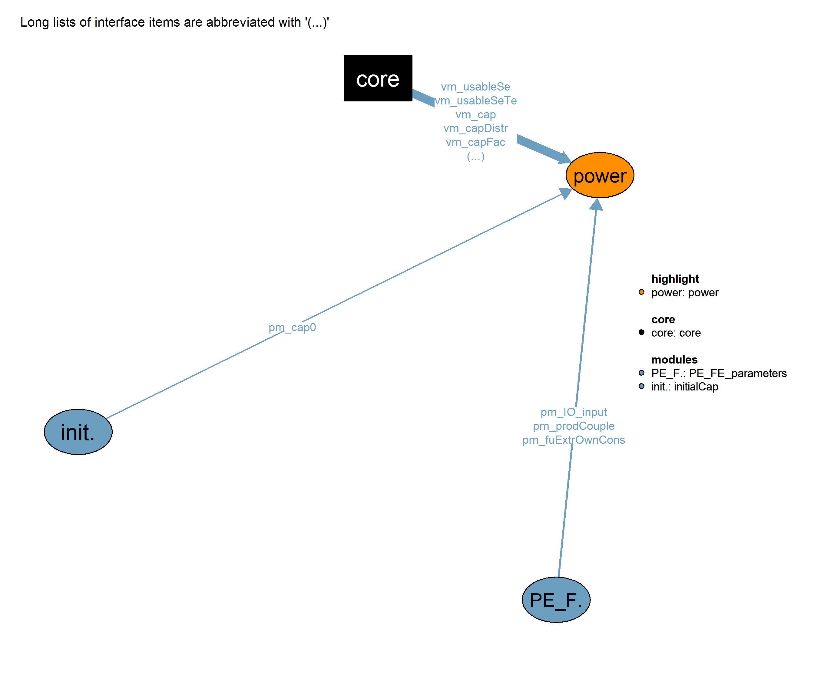
Power sector (32_power)

Description

The 32_power module determine the operation production decision for the electricity supply.

The IntC realization (Integrated Costs) assume a single electricity market balance.

The RLDC realization (Residual Load Duration Curve) distinguish different operation electricity supply decisions under four distinct load bands, plus additional peak capacity requirements.

Interfaces

Input

module inputs (A: IntC | B: RLDC)

	Description	Unit	A	B
cm_ccapturescen	carbon capture option choice			x
cm_emiscen	policy scenario choice			x
cm_nucscen	nuclear option choice			x
cm_solwindenergyscen	scenario for fluctuating renewables, 1 is reference, 2 is pessimistic with limits to fluctuating SE el share		x	x
pm_boundCapCCS (all_regi)	installed and planed capacity of CCS			x
pm_cap0 (all_regi, all_te)	standing capacity in 2005 as calculated by the initialization routine generisinical. Unit: TWa			x
pm_cf (tall, all_regi, all_te)	Installed capacity availability - capacity factor (fraction of the year that a plant is running)		x	x
pm_data (all_regi, char, all_te)	Large array for most technical parameters of technologies; more detail on the individual technical parameters can be found in the declaration of the set ‘char’		x	x
pm_dataren (all_regi, char, rlf, all_te)	Array including both regional renewable potential and capacity factor		x	x
pm_emifac (tall, all_regi, all_enty, all_enty, all_te, all_enty)	emission factor by technology for all types of emissions in emiTe			x
pm_eta_conv (tall, all_regi, all_te)	Time-dependent eta for technologies that do not have explicit time-dependant etas, still eta converges until 2050 to dataglob_values.	\(efficiency (0..1)\)	x	x
pm_fuExtrOwnCons (all_regi, all_enty, all_enty)	energy own consumption in the extraction sector with first enty being the output produced and the second enty being the input required		x	x
pm_IO_input (all_regi, all_enty, all_enty, all_te)	Energy input based on IEA data		x
pm_prodCouple (all_regi, all_enty, all_enty, all_te, all_enty)	own consumption		x	x
vm_cap (tall, all_regi, all_te, rlf)	net total capacities		x	x
vm_capDistr (tall, all_regi, all_te, rlf)	net capacities, distributed to the different grades for renewables			x
vm_capFac (ttot, all_regi, all_te)	capacity factor of conversion technologies		x	x
vm_co2CCS (ttot, all_regi, all_enty, all_enty, all_te, rlf)	all differenct ccs.	\(GtC/a\)	x	x
vm_deltaCap (tall, all_regi, all_te, rlf)	capacity additions			x
vm_demSe (ttot, all_regi, all_enty, all_enty, all_te)	se demand.	\(TWa\)	x	x
vm_demSeOth (ttot, all_regi, all_enty, all_te)	other sety demand from certain technologies, have to calculated in additional equations	\(TWa\)		x
vm_fuExtr (ttot, all_regi, all_enty, rlf)	fuel use	\(TWa\)	x	x
vm_prodFe (ttot, all_regi, all_enty, all_enty, all_te)	fe production.	\(TWa\)	x	x
vm_prodSe (tall, all_regi, all_enty, all_enty, all_te)	se production.	\(TWa\)	x	x
vm_prodSeOth (ttot, all_regi, all_enty, all_te)	other sety production from certain technologies, have to be calculated in additional equations	\(TWa\)		x
vm_usableSe (ttot, all_regi, entySe)	usable se before se2se and MP/XP (pe2se, +positive oc from pe2se, -storage losses).	\(TWa\)	x	x
vm_usableSeTe (ttot, all_regi, entySe, all_te)	usable se produced by one te (pe2se, +positive oc from pe2se, -storage losses).	\(TWa\)	x	x

Output

Realizations

(A) IntC

The IntC realization (Integrated Costs) assumes a single electricity market balance.

This module determines power system supply specific technology behavior, which sums up to the general core capacity equations to define the power sector operation and investment decisions.

Contrary to other secondary energy types in REMIND, this requires to move the electricity secondary energy balance (supply = demand) from the core to the module code.

In summary, the specific power technology equations found in this module reflect the points below.

Storage requirements are based on intermittent renewables share, synergies between different renewables production profiles and curtailment.

Additional grid capacities are calculated for high intermittent renewable capacity (solar and wind) and regional spatial differences.

Combined heat and power technologies flexibility is limited to technology and spatial observed data.

Operation reserve requirements are enforced to provide enough flexibility to the power system frequency regulation.

Hydrogen can be used to reduce renewable power curtailment and provide flexibility to the system future generation.

The IntC realization (Integrated Costs) assumes a single electricity market balance.

This module determines power system supply specific technology behavior, which sums up to the general core capacity equations to define the power sector operation and investment decisions.

Contrary to other secondary energy types in REMIND, this requires to move the electricity secondary energy balance (supply = demand) from the core to the module code.

In summary, the specific power technology equations found in this module reflect the points below.

Storage requirements are based on intermittent renewables share, synergies between different renewables production profiles and curtailment.

Additional grid capacities are calculated for high intermittent renewable capacity (solar and wind) and regional spatial differences.

Combined heat and power technologies flexibility is limited to technology and spatial observed data.

Operation reserve requirements are enforced to provide enough flexibility to the power system frequency regulation.

Hydrogen can be used to reduce renewable power curtailment and provide flexibility to the system future generation.

    v32_shStor(ttot,all_regi,all_te)                "share of seel production from renewables that needs to be stored, range 0..1 [0,1]"
    v32_storloss(ttot,all_regi,all_te)              "total energy loss from storage for a given technology [TWa]"
    v32_shSeEl(ttot,all_regi,all_te)                "new share of electricity production in % [%]"
;

\[\begin{multline*} \sum_{pe2se(enty,enty2,te)} vm\_prodSe(t,regi,enty,enty2,te) + \sum_{se2se(enty,enty2,te)} vm\_prodSe(t,regi,enty,enty2,te) + \sum_{pc2te\left(enty,entySE(enty3),te,enty2\right)}\left( pm\_prodCouple(regi,enty,enty3,te,enty2) \cdot vm\_prodSe(t,regi,enty,enty3,te) \right) + \sum_{pc2te\left(enty4,entyFE(enty5),te,enty2\right)}\left( pm\_prodCouple(regi,enty4,enty5,te,enty2) \cdot vm\_prodFe(t,regi,enty4,enty5,te) \right) + \sum_{pc2te(enty,enty3,te,enty2)}\left( \sum_{teCCS2rlf(te,rlf)}\left( pm\_prodCouple(regi,enty,enty3,te,enty2) \cdot vm\_co2CCS(t,regi,enty,enty3,te,rlf) \right) \right) = \sum_{se2fe(enty2,enty3,te)} vm\_demSe(t,regi,enty2,enty3,te) + \sum_{se2se(enty2,enty3,te)} vm\_demSe(t,regi,enty2,enty3,te) + \sum_{teVRE} v32\_storloss(t,regi,teVRE) + \sum_{pe2rlf(enty3,rlf2)}\left( \left(pm\_fuExtrOwnCons\left(regi, enty2, enty3\right) \cdot vm\_fuExtr(t,regi,enty3,rlf2)\right)\$\left(pm\_fuExtrOwnCons\left(regi, enty2, enty3\right) gt 0\right)\right)\$\left(t.val > 2005\right) !! don't use in 2005 because this demand is not contained in 05\_initialCap \end{multline*}\]

\[\begin{multline*} vm\_usableSe(t,regi,entySe) = \sum_{pe2se(enty,entySe,te)} vm\_prodSe(t,regi,enty,entySe,te) + \sum_{se2se(enty,entySe,te)} vm\_prodSe(t,regi,enty,entySe,te) + \sum_{pc2te\left(entyPe,entySe(enty3),te,entySe\right)\$\left(pm\_prodCouple(regi,entyPe,enty3,te,entySe) gt 0\right)}\left( pm\_prodCouple(regi,entyPe,enty3,te,entySe) \cdot vm\_prodSe(t,regi,entyPe,enty3,te) \right) - \sum_{teVRE} v32\_storloss(t,regi,teVRE) \end{multline*}\]

\[\begin{multline*} vm\_usableSeTe(t,regi,entySe,te) = \sum_{pe2se(enty,entySe,te)} vm\_prodSe(t,regi,enty,entySe,te) + \sum_{se2se(enty,entySe,te)} vm\_prodSe(t,regi,enty,entySe,te) + \sum_{pc2te\left(enty,entySe(enty3),te,entySe\right)\$\left(pm\_prodCouple(regi,enty,enty3,te,entySe) gt 0\right)}\left( pm\_prodCouple(regi,enty,enty3,te,entySe) \cdot vm\_prodSe(t,regi,enty,enty3,te) \right) - \sum_{teVRE\$sameas(te,teVRE)} v32\_storloss(t,regi,teVRE) \end{multline*}\]

\[\begin{multline*} \sum_{VRE2teStor(teVRE,teStor)} v32\_storloss(t,regi,teVRE) \cdot \frac{ pm\_eta\_conv(t,regi,teStor) }{ \left( 1 - pm\_eta\_conv(t,regi,teStor)\right) } \leq \sum_{te2rlf(teStor,rlf)}\left( vm\_capFac(t,regi,teStor) \cdot pm\_dataren(regi,"nur",rlf,teStor) \cdot vm\_cap(t,regi,teStor,rlf) \right) \end{multline*}\]

\[\begin{multline*} vm\_cap(t,regi,"h2turbVRE","1") = \sum_{te\$testor(te)}\left( p32\_storageCap(te,"h2turbVREcapratio") \cdot vm\_cap(t,regi,te,"1") \right) \end{multline*}\]

\[\begin{multline*} vm\_cap(t,regi,"elh2VRE","1") = \sum_{te\$testor(te)}\left( p32\_storageCap(te,"elh2VREcapratio") \cdot vm\_cap(t,regi,te,"1") \right) \end{multline*}\]

\[\begin{multline*} \sum_{pe2se\left(enty,"seel",teChp(te)\right)} vm\_prodSe(t,regi,enty,"seel",te) \leq p32\_shCHP(regi,"bscu") \cdot \sum_{pe2se(enty,"seel",te)} vm\_prodSe(t,regi,enty,"seel",te) \end{multline*}\]

\[\begin{multline*} \frac{\frac{ vm\_cap(t,regi,"gridwind",'1') !! Technology is now parameterized to yield marginal costs of ~3.5\$}{MWh VRE electricity }}{ p32\_grid\_factor(regi) !! It is assumed that large regions require higher grid investment } \geq vm\_prodSe(t,regi,"pesol","seel","spv") + vm\_prodSe(t,regi,"pesol","seel","csp") + 1.5 \cdot vm\_prodSe(t,regi,"pewin","seel","wind") !! wind has larger variations accross space, so adding grid is more important for wind \left(result of REMIX runs for ADVANCE project\right) \end{multline*}\]

\[\begin{multline*} \frac{ v32\_shSeEl(t,regi,teVRE) }{ 100 } \cdot vm\_usableSe(t,regi,"seel") = vm\_usableSeTe(t,regi,"seel",teVRE) \end{multline*}\]

\[\begin{multline*} v32\_shStor(t,regi,teVRE) \geq p32\_factorStorage(regi,teVRE) \cdot 100 \cdot \left( \left(1.e-10 +\frac{ \left(v32\_shSeEl(t,regi,teVRE)+\frac{ \sum_{VRE2teVRElinked(teVRE,teVRE2)} v32\_shSeEl(t,regi,teVRE2) }{s32\_storlink}\right)}{100 }\right) ^{ p32\_storexp(regi,teVRE) !! offset of 1.e}-10 for numerical reasons: gams doesn't like 0 if the exponent is not integer - \left(1.e-10 ^{ p32\_storexp(regi,teVRE) }\right) !! offset correction - 0.07 !! first 7\% of VRE share bring no negative effects \right) \end{multline*}\]

\[\begin{multline*} v32\_storloss(t,regi,teVRE) = \frac{ v32\_shStor(t,regi,teVRE) }{ 93 !! corrects for the 7\%}-shift in v32\_shStor: at 100\% the value is correct again \cdot \sum_{VRE2teStor(teVRE,teStor)}\left(\frac{ \left(1 - pm\_eta\_conv(t,regi,teStor) \right) }{ pm\_eta\_conv(t,regi,teStor) }\right) \cdot vm\_usableSeTe(t,regi,"seel",teVRE) \end{multline*}\]

\[\begin{multline*} vm\_usableSe(t,regi,"seel") \leq \sum_{pe2se(enty,"seel",te)\$\left(NOT teVRE(te)\right)}\left( pm\_data(regi,"flexibility",te) \cdot vm\_prodSe(t,regi,enty,"seel",te) \right) + \sum_{se2se(enty,"seel",te)\$\left(NOT teVRE(te)\right)}\left( pm\_data(regi,"flexibility",te) \cdot vm\_prodSe(t,regi,enty,"seel",te) \right) + \sum_{pe2se(enty,"seel",teVRE)}\left( pm\_data(regi,"flexibility",teVRE) \cdot \left(vm\_prodSe(t,regi,enty,"seel",teVRE)-v32\_storloss(t,regi,teVRE)\right) \right) + \sum_{pe2se(enty,"seel",teVRE)}\left( \sum_{VRE2teStor(teVRE,teStor)}\left( pm\_data(regi,"flexibility",teStor) \cdot \left(vm\_prodSe(t,regi,enty,"seel",teVRE)-v32\_storloss(t,regi,teVRE)\right) \right) \right) \end{multline*}\]

\[\begin{multline*} vm\_usableSeTe(t,regi,"seel","spv") + vm\_usableSeTe(t,regi,"seel","wind") + vm\_usableSeTe(t,regi,"seel","csp") \leq 0.2 \cdot vm\_usableSe(t,regi,"seel") \end{multline*}\]

The IntC realization (Integrated Costs) assumes a single electricity market balance.

This module determines power system supply specific technology behavior, which sums up to the general core capacity equations to define the power sector operation and investment decisions.

Contrary to other secondary energy types in REMIND, this requires to move the electricity secondary energy balance (supply = demand) from the core to the module code.

In summary, the specific power technology equations found in this module reflect the points below.

Storage requirements are based on intermittent renewables share, synergies between different renewables production profiles and curtailment.

Additional grid capacities are calculated for high intermittent renewable capacity (solar and wind) and regional spatial differences.

Combined heat and power technologies flexibility is limited to technology and spatial observed data.

Operation reserve requirements are enforced to provide enough flexibility to the power system frequency regulation.

Hydrogen can be used to reduce renewable power curtailment and provide flexibility to the system future generation.

Limitations There are no known limitations.

(B) RLDC

The RLDC realization (Residual Load Duration Curve) distinguish different operation electricity supply decisions under four distinct load bands, plus additional peak capacity requirements.

This module determine power system supply specific technology behavior, which summs up to the general core capacity equations to define the power sector operation and investment decisions.

Contrary to other secondary energies in REMIND, this requires to move the electricity secondary energy balance (supply = demand) from the core to the module code.

The residual load duration curve is obtained after discounting intermittent renewables generation (solar and wind) from the total demand.

An exogenous unit commitment model (DIMES) is used to estimate a third degree fitting curve for each load band representing the intermittent renewables generation contribution at different renewable penetration shares in the system.

Curtailament is defined using the same process - a per load band third degree fitting curve that determines the curtailment based on the renewables share.

Dispatchable power generation technologies have their capacity factor endogenously determined by the use in the distinct load bands.

Short term storage is dependable of wind and solar penetration shares and estimated exogenously to a third degree fitting curve.

A reserve margin capacity is required to be provided by dispatchable technologies only. The reserve margin size is determined by the peak capacity that is also estimated exogenously for different levels of renewables penetration in the system.

CSP co-firing with H2 or other gases is included. Self-correlation and PV correlation inside each load bands are considered.

Hydrogen can be used to reduce renewable power curtailment and provide flexibility to the system future generation.

Hydropower load band flexibility is limited due to run-of-river power plants and water use regulation constraints.

Combined heat and power technologies flexibility is limited to technology and spatial observed data.

Additional grid capacities are calculated for high intermittent renewable capacity (solar and wind) and regional spatial differences.

The RLDC realization (Residual Load Duration Curve) distinguish different operation electricity supply decisions under four distinct load bands, plus additional peak capacity requirements.

This module determine power system supply specific technology behavior, which summs up to the general core capacity equations to define the power sector operation and investment decisions.

Contrary to other secondary energies in REMIND, this requires to move the electricity secondary energy balance (supply = demand) from the core to the module code.

The residual load duration curve is obtained after discounting intermittent renewables generation (solar and wind) from the total demand.

An exogenous unit commitment model (DIMES) is used to estimate a third degree fitting curve for each load band representing the intermittent renewables generation contribution at different renewable penetration shares in the system.

Curtailament is defined using the same process - a per load band third degree fitting curve that determines the curtailment based on the renewables share.

Dispatchable power generation technologies have their capacity factor endogenously determined by the use in the distinct load bands.

Short term storage is dependable of wind and solar penetration shares and estimated exogenously to a third degree fitting curve.

A reserve margin capacity is required to be provided by dispatchable technologies only. The reserve margin size is determined by the peak capacity that is also estimated exogenously for different levels of renewables penetration in the system.

CSP co-firing with H2 or other gases is included. Self-correlation and PV correlation inside each load bands are considered.

Hydrogen can be used to reduce renewable power curtailment and provide flexibility to the system future generation.

Hydropower load band flexibility is limited due to run-of-river power plants and water use regulation constraints.

Combined heat and power technologies flexibility is limited to technology and spatial observed data.

Additional grid capacities are calculated for high intermittent renewable capacity (solar and wind) and regional spatial differences.

\[\begin{multline*} v32\_scaleCap(t,regi) \cdot p32\_capFacDem(regi) + \sum_{pc2te\left(enty,entySE(enty3),te,enty2\right)}\left( pm\_prodCouple(regi,enty,enty3,te,enty2) \cdot vm\_prodSe(t,regi,enty,enty3,te) \right) + \sum_{pc2te\left(enty4,entyFE(enty5),te,enty2\right)}\left( pm\_prodCouple(regi,enty4,enty5,te,enty2) \cdot vm\_prodFe(t,regi,enty4,enty5,te) \right) + \sum_{pc2te(enty,enty3,te,enty2)}\left( \sum_{teCCS2rlf(te,rlf)}\left( pm\_prodCouple(regi,enty,enty3,te,enty2) \cdot vm\_co2CCS(t,regi,enty,enty3,te,rlf) \right) \right) = \sum_{se2fe(enty2,enty3,te)} vm\_demSe(t,regi,enty2,enty3,te) + \sum_{se2se(enty2,enty3,te)} vm\_demSe(t,regi,enty2,enty3,te) + \sum_{pe2rlf(enty3,rlf2)}\left( \left(pm\_fuExtrOwnCons\left(regi, enty2, enty3\right) \cdot vm\_fuExtr(t,regi,enty3,rlf2)\right)\$\left(pm\_fuExtrOwnCons\left(regi, enty2, enty3\right) gt 0\right)\right)\$\left(t.val > 2005\right) !! don't use in 2005 because this demand is not contained in 05\_initialCap \end{multline*}\]

\[\begin{multline*} vm\_usableSe(t,regi,entySe) = \sum_{pe2se(enty,entySe,te)} vm\_prodSe(t,regi,enty,entySe,te) + \sum_{se2se(enty,entySe,te)} vm\_prodSe(t,regi,enty,entySe,te) + \sum_{pc2te\left(entyPe,entySe(enty3),te,entySe\right)\$\left(pm\_prodCouple(regi,entyPe,enty3,te,entySe) gt 0\right)}\left( pm\_prodCouple(regi,entyPe,enty3,te,entySe) \cdot vm\_prodSe(t,regi,entyPe,enty3,te) \right) \end{multline*}\]

\[\begin{multline*} vm\_usableSeTe(t,regi,entySe,te) = \sum_{pe2se(enty,entySe,te)} vm\_prodSe(t,regi,enty,entySe,te) + \sum_{se2se(enty,entySe,te)} vm\_prodSe(t,regi,enty,entySe,te) + \sum_{pc2te\left(enty,entySe(enty3),te,entySe\right)\$\left(pm\_prodCouple(regi,enty,enty3,te,entySe) gt 0\right)}\left( pm\_prodCouple(regi,enty,enty3,te,entySe) \cdot vm\_prodSe(t,regi,enty,enty3,te) \right) \end{multline*}\]

\[\begin{multline*} v32\_shTh(t,regi,teVRE) = \frac{ \sum_{pe2se(entyPe,"seel",teVRE)} vm\_prodSe(t,regi,entyPe,"seel",teVRE) }{ \left( v32\_scaleCap(t,regi) \cdot p32\_capFacDem(regi) + \sum_{pc2te\left(enty,entySE(enty3),te,enty2\right)}\left( pm\_prodCouple(regi,enty,enty3,te,enty2) \cdot vm\_prodSe(t,regi,enty,enty3,te) \right) + \sum_{pc2te\left(enty4,entyFE(enty5),te,enty2\right)}\left( pm\_prodCouple(regi,enty4,enty5,te,enty2) \cdot vm\_prodFe(t,regi,enty4,enty5,te) \right) + \sum_{pc2te(enty,enty3,te,enty2)}\left( \sum_{teCCS2rlf(te,rlf)}\left( pm\_prodCouple(regi,enty,enty3,te,enty2) \cdot vm\_co2CCS(t,regi,enty,enty3,te,rlf) \right) \right) \right) } \end{multline*}\]

\[\begin{multline*} !! scale the capacities of all technologies explicitly represented in the RLDCs \sum_{tese2rlf(te,rlf)} vm\_cap(t,regi,te,rlf) = v32\_scaleCap(t,regi) \cdot \left( \sum\left(LoB, v32\_capLoB(t,regi,te,LoB) \right) + v32\_capER(t,regi,te) \right) \end{multline*}\]

\[\begin{multline*} v32\_curt(t,regi) = \sum_{pe2se(entyPe,"seel",teVRE)} vm\_prodSe(t,regi,entyPe,"seel",teVRE) !! total theoretical VRE production - v32\_scaleCap(t,regi) \cdot \left( p32\_capFacDem(regi) - \sum_{LoB}\left( p32\_capFacLoB(LoB) \cdot v32\_LoBheight(t,regi,LoB) \right) \right) !! minus the actually used VRE production, namely the difference between a system without and a system with VRE + v32\_overProdCF(t,regi,"csp") \cdot vm\_cap(t,regi,"csp","1") !! add the unused CSP production that is not reflected in seprod \end{multline*}\]

\[\begin{multline*} !! calculate curtailment as fitted from the DIMES-Results v32\_curtFit(t,regi) !! v32\_curtFit can go below 0 = p32\_curtOn(regi) \cdot \left( p32\_RLDCcoeff(regi,"p00","curtShVRE") + p32\_RLDCcoeff(regi,"p10","curtShVRE") \cdot v32\_shTh(t,regi,"wind")\$teVRE("wind") + p32\_RLDCcoeff(regi,"p01","curtShVRE") \cdot \left( v32\_shTh(t,regi,"spv")\$teVRE("spv") + v32\_shTh(t,regi,"csp")\$teVRE("csp") \right) + p32\_RLDCcoeff(regi,"p20","curtShVRE") \cdot v32\_shTh(t,regi,"wind")\$teVRE("wind") ^{ 2 }+ p32\_RLDCcoeff(regi,"p11","curtShVRE") \cdot v32\_shTh(t,regi,"wind")\$teVRE("wind") \cdot \left( v32\_shTh(t,regi,"spv")\$teVRE("spv") + v32\_shTh(t,regi,"csp")\$teVRE("csp") \right) + p32\_RLDCcoeff(regi,"p02","curtShVRE") \cdot \left( v32\_shTh(t,regi,"spv")\$teVRE("spv") + v32\_shTh(t,regi,"csp")\$teVRE("csp") \right) ^{ 2 }+ p32\_RLDCcoeff(regi,"p30","curtShVRE") \cdot v32\_shTh(t,regi,"wind")\$teVRE("wind") ^{ 3 }+ p32\_RLDCcoeff(regi,"p21","curtShVRE") \cdot v32\_shTh(t,regi,"wind")\$teVRE("wind") ^{ 2 } \cdot \left( v32\_shTh(t,regi,"spv")\$teVRE("spv") + v32\_shTh(t,regi,"csp")\$teVRE("csp") \right) + p32\_RLDCcoeff(regi,"p12","curtShVRE") \cdot v32\_shTh(t,regi,"wind")\$teVRE("wind") \cdot \left( v32\_shTh(t,regi,"spv")\$teVRE("spv") + v32\_shTh(t,regi,"csp")\$teVRE("csp") \right) ^{ 2 }+ p32\_RLDCcoeff(regi,"p03","curtShVRE") \cdot \left( v32\_shTh(t,regi,"spv")\$teVRE("spv") + v32\_shTh(t,regi,"csp")\$teVRE("csp") \right) ^{ 3 }\right) \end{multline*}\]

q32_curtFitwCSP(t,regi)..
    v32_curt(t,regi)   
    =e=  
    ( v32_curtFit(t,regi) + 0.02 ) * sum(pe2se(entyPe,"seel",teVRE), vm_prodSe(t,regi,entyPe,"seel",teVRE) )  !! add 2% of VRE prod. ot curtailment to represent grid losses - comes from the comparison with REMIX
    + v32_overProdCF(t,regi,"csp") * vm_cap(t,regi,"csp","1")
    + v32_CurtModelminusFit(t,regi)  * sum(pe2se(entyPe,"seel",teVRE), vm_prodSe(t,regi,entyPe,"seel",teVRE) )       !! this is a positive slack variable that shows how much curtailment due to discretization of RLDC boxes is larger than fitted curtailment -> to move to ex-post
$if %cm_Full_Integration% == "on" + v32_FullIntegrationSlack(t,regi)
;

\[\begin{multline*} v32\_LoBheightCumExact(t,regi,LoB) = p32\_RLDCcoeff(regi,"p00",LoB) + p32\_RLDCcoeff(regi,"p10",LoB) \cdot v32\_shTh(t,regi,"wind")\$teVRE("wind") + p32\_RLDCcoeff(regi,"p01",LoB) \cdot \left( v32\_shTh(t,regi,"spv")\$teVRE("spv") + v32\_shTh(t,regi,"csp")\$teVRE("csp") \right) + p32\_RLDCcoeff(regi,"p20",LoB) \cdot v32\_shTh(t,regi,"wind")\$teVRE("wind") ^{ 2 }+ p32\_RLDCcoeff(regi,"p11",LoB) \cdot v32\_shTh(t,regi,"wind")\$teVRE("wind") \cdot \left( v32\_shTh(t,regi,"spv")\$teVRE("spv") + v32\_shTh(t,regi,"csp")\$teVRE("csp") \right) + p32\_RLDCcoeff(regi,"p02",LoB) \cdot \left( v32\_shTh(t,regi,"spv")\$teVRE("spv") + v32\_shTh(t,regi,"csp")\$teVRE("csp") \right) ^{ 2 }+ p32\_RLDCcoeff(regi,"p30",LoB) \cdot v32\_shTh(t,regi,"wind")\$teVRE("wind") ^{ 3 }+ p32\_RLDCcoeff(regi,"p21",LoB) \cdot v32\_shTh(t,regi,"wind")\$teVRE("wind") ^{ 2 } \cdot \left( v32\_shTh(t,regi,"spv")\$teVRE("spv") + v32\_shTh(t,regi,"csp")\$teVRE("csp") \right) + p32\_RLDCcoeff(regi,"p12",LoB) \cdot v32\_shTh(t,regi,"wind")\$teVRE("wind") \cdot \left( v32\_shTh(t,regi,"spv")\$teVRE("spv") + v32\_shTh(t,regi,"csp")\$teVRE("csp") \right) ^{ 2 }+ p32\_RLDCcoeff(regi,"p03",LoB) \cdot \left( v32\_shTh(t,regi,"spv")\$teVRE("spv") + v32\_shTh(t,regi,"csp")\$teVRE("csp") \right) ^{ 3 } \end{multline*}\]

\[\begin{multline*} !! introduce slack so that v32\_LoBheightCum stay > 0 v32\_LoBheightCum(t,regi,LoB) \geq v32\_LoBheightCumExact(t,regi,LoB) \end{multline*}\]

\[\begin{multline*} !! individual load band height - the difference between the cumulated heights v32\_LoBheight(t,regi,LoB) \geq \left( v32\_LoBheightCum(t,regi,LoB) - v32\_LoBheightCum(t,regi,LoB+1)\$\left(LoB.val < card(LoB)\right) \right) \cdot \left( 1\$\left(LoB.val < card(LoB)\right) + \left(\frac{ 1 }{ p32\_capFacLoB(LoB) }\right)\$\left(LoB.val = card(LoB)\right) \right) !! upscale the height of the base-load band to represent the fact that the fit was done with 8760 hours, while no plant runs longer than 7500 hours \left(CF = 0.86\right) \end{multline*}\]

\[\begin{multline*} \sum_{teRLDCDisp} v32\_capLoB(t,regi,teRLDCDisp,LoB) = v32\_LoBheight(t,regi,LoB) \end{multline*}\]

\[\begin{multline*} vm\_capFac(t,regi,te) = \frac{ \left( \sum_{LoB}\left( \left( p32\_capFacLoB(LoB)\$\left( \left(LoB.val <> 4\right) OR NOT sameas(te,"csp") \right) +\frac{\frac{ \left(\frac{4}{3 } \cdot p32\_avCapFac(t,regi,"csp")\right)\$\left( \left(LoB.val eq 4\right) \& sameas(te,"csp") \right) !! 4}{3 is a factor for the upscaling from SM3}}{\frac{12h to SM4}{16h storage }}\right) \cdot v32\_capLoB(t,regi,te,LoB) \right) + v32\_capER(t,regi,te) \cdot 0.01 !! the early retired capacities v32\_capER are weighted with 1\% to represent that they run at least 100h per year \right) }{ \left(\sum_{LoB} v32\_capLoB(t,regi,te,LoB) + v32\_capER(t,regi,te) + 1e-9\right) } \end{multline*}\]

\[\begin{multline*} \frac{!! make sure that for dispatchable renewable plants, the average nur is larger than the resulting capFac \sum_{teRe2rlfDetail(te,rlf)}\left( pm\_dataren(regi,"nur",rlf,te) \cdot vm\_capDistr(t,regi,te,rlf) \right) }{ \left( vm\_cap(t,regi,te,"1") + 1e-10 \right) }+ 3e-5 !! the 1e-5 allows for slightly larger capacity factors, but does not have a large influence, and prevents some infeasibilities \geq vm\_capFac(t,regi,te) + v32\_overProdCF(t,regi,te) \end{multline*}\]

\[\begin{multline*} vm\_cap(t,regi,"storspv","1") \geq v32\_scaleCap(t,regi) \cdot \left( p32\_RLDCcoeff(regi,"p00","STScost") + p32\_RLDCcoeff(regi,"p10","STScost") \cdot v32\_shTh(t,regi,"wind")\$teVRE("wind") + p32\_RLDCcoeff(regi,"p01","STScost") \cdot \left( v32\_shTh(t,regi,"spv")\$teVRE("spv") + v32\_shTh(t,regi,"csp")\$teVRE("csp") \right) + p32\_RLDCcoeff(regi,"p20","STScost") \cdot v32\_shTh(t,regi,"wind")\$teVRE("wind") ^{ 2 }+ p32\_RLDCcoeff(regi,"p11","STScost") \cdot v32\_shTh(t,regi,"wind")\$teVRE("wind") \cdot \left( v32\_shTh(t,regi,"spv")\$teVRE("spv") + v32\_shTh(t,regi,"csp")\$teVRE("csp") \right) + p32\_RLDCcoeff(regi,"p02","STScost") \cdot \left( v32\_shTh(t,regi,"spv")\$teVRE("spv") + v32\_shTh(t,regi,"csp")\$teVRE("csp") \right) ^{ 2 }+ p32\_RLDCcoeff(regi,"p30","STScost") \cdot v32\_shTh(t,regi,"wind")\$teVRE("wind") ^{ 3 }+ p32\_RLDCcoeff(regi,"p21","STScost") \cdot v32\_shTh(t,regi,"wind")\$teVRE("wind") ^{ 2 } \cdot \left( v32\_shTh(t,regi,"spv")\$teVRE("spv") + v32\_shTh(t,regi,"csp")\$teVRE("csp") \right) + p32\_RLDCcoeff(regi,"p12","STScost") \cdot v32\_shTh(t,regi,"wind")\$teVRE("wind") \cdot \left( v32\_shTh(t,regi,"spv")\$teVRE("spv") + v32\_shTh(t,regi,"csp")\$teVRE("csp") \right) ^{ 2 }+ p32\_RLDCcoeff(regi,"p03","STScost") \cdot \left( v32\_shTh(t,regi,"spv")\$teVRE("spv") + v32\_shTh(t,regi,"csp")\$teVRE("csp") \right) ^{ 3 }\right) \end{multline*}\]

\[\begin{multline*} v32\_peakCap(t,regi) = p32\_RLDCcoeff(regi,"p00","peak") + p32\_RLDCcoeff(regi,"p10","peak") \cdot v32\_shTh(t,regi,"wind")\$teVRE("wind") + p32\_RLDCcoeff(regi,"p01","peak") \cdot \left( v32\_shTh(t,regi,"spv")\$teVRE("spv") + v32\_shTh(t,regi,"csp")\$teVRE("csp") \right) + p32\_RLDCcoeff(regi,"p20","peak") \cdot v32\_shTh(t,regi,"wind")\$teVRE("wind") ^{ 2 }+ p32\_RLDCcoeff(regi,"p11","peak") \cdot v32\_shTh(t,regi,"wind")\$teVRE("wind") \cdot \left( v32\_shTh(t,regi,"spv")\$teVRE("spv") + v32\_shTh(t,regi,"csp")\$teVRE("csp") \right) + p32\_RLDCcoeff(regi,"p02","peak") \cdot \left( v32\_shTh(t,regi,"spv")\$teVRE("spv") + v32\_shTh(t,regi,"csp")\$teVRE("csp") \right) ^{ 2 }+ p32\_RLDCcoeff(regi,"p30","peak") \cdot v32\_shTh(t,regi,"wind")\$teVRE("wind") ^{ 3 }+ p32\_RLDCcoeff(regi,"p21","peak") \cdot v32\_shTh(t,regi,"wind")\$teVRE("wind") ^{ 2 } \cdot \left( v32\_shTh(t,regi,"spv")\$teVRE("spv") + v32\_shTh(t,regi,"csp")\$teVRE("csp") \right) + p32\_RLDCcoeff(regi,"p12","peak") \cdot v32\_shTh(t,regi,"wind")\$teVRE("wind") \cdot \left( v32\_shTh(t,regi,"spv")\$teVRE("spv") + v32\_shTh(t,regi,"csp")\$teVRE("csp") \right) ^{ 2 }+ p32\_RLDCcoeff(regi,"p03","peak") \cdot \left( v32\_shTh(t,regi,"spv")\$teVRE("spv") + v32\_shTh(t,regi,"csp")\$teVRE("csp") \right) ^{ 3 } \end{multline*}\]

\[\begin{multline*} \sum_{teRLDCDisp(te)\$\left(NOT sameas(te,"hydro")\right)}\left( \sum_{tese2rlf(te,rlf)} vm\_cap(t,regi,te,rlf) \right) + 0.8 \cdot vm\_cap(t,regi,"hydro","1") !! to represent that it is not fully dispatchable, hydro counts only with 80\% of its installed capacity towards peak capacity \geq v32\_scaleCap(t,regi) \cdot \left( v32\_peakCap(t,regi) + p32\_ResMarg(t,regi) \right) \end{multline*}\]

q32_H2cofiring(t,regi)$(t.val > 2010)..
    vm_demSeOth(t,regi,"seh2","csp")                 !! cofiring of h2 to csp 
    + vm_demSeOth(t,regi,"segabio","csp")               !! cofiring of gas to csp 
    + vm_demSeOth(t,regi,"segafos","csp")
$if %cm_Full_Integration% == "on"  + 1e6
    =g= 
    v32_H2cof_PVsh(t,regi)
    + v32_H2cof_Lob4(t,regi)
    + v32_H2cof_Lob3(t,regi)
    + v32_H2cof_CSPsh(t,regi)
;

\[\begin{multline*} v32\_H2cof\_Lob3(t,regi) \geq \frac{\frac{ 1}{0.4 !! 1}}{0.4 is the efficiency of the H2 turbine }- to convert from produced electricity to used H2 \cdot v32\_scaleCap(t,regi) !! all the later numbers are relative to peak, and need to be rescaled to full system size \cdot v32\_capLoB(t,regi,"csp","3") !! each unit of csp in baseload needs H2 cofiring \cdot \left( p32\_capFacLoB("3") - p32\_avCapFac(t,regi,"csp") \right) !! the co-firing is only needed for the residual of baseload after avCapFac. CapLob \cdot DiffCapfac = produced electricity \end{multline*}\]

\[\begin{multline*} v32\_H2cof\_Lob4(t,regi) \geq \frac{\frac{ 1}{0.4 !! 1}}{0.4 is the efficiency of the H2 turbine }- to convert from produced electricity to used H2 \cdot v32\_scaleCap(t,regi) \cdot v32\_capLoB(t,regi,"csp","4") !! each unit of csp in baseload needs H2 cofiring \cdot \frac{\frac{ \left( p32\_capFacLoB("4") -\frac{ 4}{3 } \cdot p32\_avCapFac(t,regi,"csp") \right) !! 4}{3 is the factor for the upscaling from SM3}}{\frac{12h to SM4}{16h storage }} \end{multline*}\]

\[\begin{multline*} !! more CSP cofiring if lots of PV is used \left(correlation between PV and CSP\right) v32\_H2cof\_PVsh(t,regi) = \frac{\frac{ 1}{0.4 !! 1}}{0.4 is the efficiency of the H2 turbine }- to convert from produced electricity to used H2 \cdot v32\_scaleCap(t,regi) \cdot 0.5 \cdot vm\_cap(t,regi,"csp","1") \cdot \left(0.65 - p32\_avCapFac(t,regi,"csp") \right) \cdot v32\_shTh(t,regi,"spv") \end{multline*}\]

\[\begin{multline*} !! more CSP cofiring if lots of CSP is used \left(self-correlation of CSP\right) v32\_H2cof\_CSPsh(t,regi) = \frac{\frac{ 1}{0.4 !! 1}}{0.4 is the efficiency of the H2 turbine }- to convert from produced electricity to used H2 \cdot v32\_scaleCap(t,regi) \cdot vm\_cap(t,regi,"csp","1") \cdot \left(0.65 - p32\_avCapFac(t,regi,"csp") \right) \cdot v32\_shTh(t,regi,"csp") \end{multline*}\]

\[\begin{multline*} \frac{ vm\_cap(t,regi,"h2curt","1") }{ v32\_scaleCap(t,regi) !! 0.5 for area of a triangle } \leq v32\_sqrtCurt(t,regi) !! 0.5 as only half of the curtailment can be used \end{multline*}\]

\[\begin{multline*} pm\_eta\_conv(t,regi,"h2curt") \cdot vm\_cap(t,regi,"h2curt","1") \cdot \frac{ 2}{3 } \cdot v32\_sqrtCurt(t,regi) \geq vm\_prodSeOth(t,regi,"seh2","h2curt") \end{multline*}\]

\[\begin{multline*} v32\_sqrtCurt(t,regi) = sqrt\left(\frac{ 2}{3 } \cdot \left(\frac{\frac{ v32\_curt(t,regi) }{ v32\_scaleCap(t,regi) }}{ p32\_capFacDem(regi) }+ 1e-6 \right) \right) \end{multline*}\]

\[\begin{multline*} !! require that at least 20\% of the hydro are in baseload \left(counting as run-of-river\right). This may lead to Baseload being higher than required by the RLDC, and therefore realistic curtailment p32\_capFacLoB("4") \cdot v32\_capLoB(t,regi,"hydro","4") \geq 0.2 \cdot \sum_{LoB}\left( p32\_capFacLoB(LoB) \cdot v32\_capLoB(t,regi,"hydro",LoB) \right) \end{multline*}\]

\[\begin{multline*} \sum_{pe2se\left(enty,"seel",teChp(te)\right)} vm\_prodSe(t,regi,enty,"seel",te) \leq p32\_shCHP(regi,"bscu") \cdot \sum_{pe2se(enty,"seel",te)} vm\_prodSe(t,regi,enty,"seel",te) \end{multline*}\]

\[\begin{multline*} \frac{\frac{ vm\_cap(t,regi,"gridwind",'1') !! Technology is now parameterized to yield marginal costs of ~3.5\$}{MWh VRE electricity }}{ p32\_grid\_factor(regi) !! It is assumed that large regions require higher grid investment } \geq vm\_prodSe(t,regi,"pesol","seel","spv") + vm\_prodSe(t,regi,"pesol","seel","csp") + 1.5 \cdot vm\_prodSe(t,regi,"pewin","seel","wind") !! wind has larger variations accross space, so adding grid is more important for wind \left(result of REMIX runs for ADVANCE project\right) \end{multline*}\]

\[\begin{multline*} vm\_usableSeTe(t,regi,"seel","spv") + vm\_usableSeTe(t,regi,"seel","wind") + vm\_usableSeTe(t,regi,"seel","csp") \leq 0.2 \cdot vm\_usableSe(t,regi,"seel") \end{multline*}\]

The RLDC realization (Residual Load Duration Curve) distinguish different operation electricity supply decisions under four distinct load bands, plus additional peak capacity requirements.

This module determine power system supply specific technology behavior, which summs up to the general core capacity equations to define the power sector operation and investment decisions.

Contrary to other secondary energies in REMIND, this requires to move the electricity secondary energy balance (supply = demand) from the core to the module code.

The residual load duration curve is obtained after discounting intermittent renewables generation (solar and wind) from the total demand.

An exogenous unit commitment model (DIMES) is used to estimate a third degree fitting curve for each load band representing the intermittent renewables generation contribution at different renewable penetration shares in the system.

Curtailament is defined using the same process - a per load band third degree fitting curve that determines the curtailment based on the renewables share.

Dispatchable power generation technologies have their capacity factor endogenously determined by the use in the distinct load bands.

Short term storage is dependable of wind and solar penetration shares and estimated exogenously to a third degree fitting curve.

A reserve margin capacity is required to be provided by dispatchable technologies only. The reserve margin size is determined by the peak capacity that is also estimated exogenously for different levels of renewables penetration in the system.

CSP co-firing with H2 or other gases is included. Self-correlation and PV correlation inside each load bands are considered.

Hydrogen can be used to reduce renewable power curtailment and provide flexibility to the system future generation.

Hydropower load band flexibility is limited due to run-of-river power plants and water use regulation constraints.

Combined heat and power technologies flexibility is limited to technology and spatial observed data.

Additional grid capacities are calculated for high intermittent renewable capacity (solar and wind) and regional spatial differences.

Limitations There are no known limitations.

Definitions

Objects

module-internal objects (A: IntC | B: RLDC)

	Description	Unit	A	B
f32_factorStorage (all_regi, all_te)	multiplicative factor that scales total curtailment and storage requirements up or down in different regions for different technologies (e.g. down for PV in regions where high solar radiation coincides with high electricity demand)		x
f32_RLDC_Coeff_LoB (all_regi, RLDCbands, PolyCoeff)	RLDC coefficients for combined Wind-Solar Polynomial			x
f32_RLDC_Coeff_Peak (all_regi, RLDCbands, PolyCoeff)	RLDC coefficients for combined Wind-Solar Polynomial			x
f32_shCHP (all_regi, char)	upper boundary of chp electricity generation		x	x
f32_storageCap (char, all_te)	multiplicative factor between dummy seel<–>h2 technologies and storXXX technologies		x
p32_avCapFac (ttot, all_regi, all_te)	Average load factor (Nur) of the first 5 grades of a technology			x
p32_capFacDem (all_regi)	Average demand factor of a power sector	\(0,1\)		x
p32_capFacLoB (LoB)	Capacity factor of a load band	\(0,1\)		x
p32_curtOn (all_regi)	Control variable for curtailment fitted from the DIMES-Results			x
p32_factorStorage (all_regi, all_te)	multiplicative factor that scales total curtailment and storage requirements up or down in different regions for different technologies (e.g. down for PV in regions where high solar radiation coincides with high electricity demand)		x
p32_grid_factor (all_regi)	multiplicative factor that scales total grid requirements down in comparatively small or homogeneous regions like Japan, Europe or India		x	x
p32_gridexp (all_regi, all_te)	exponent that determines how grid requirement per kW increases with market share of wind and solar. 1 means specific marginal costs increase linearly		x
p32_LoBheight0 (all_regi, LoB)	Load band heights at 0% VRE share (declared here, on the data input file, because it is only used for the p32_capFacDem definition)	\(0,1\)		x
p32_ResMarg (ttot, all_regi)	Reserve margin as markup on actual peak capacity	\(0,1\)		x
p32_RLDCcoeff (all_regi, PolyCoeff, RLDCbands)	Coefficients for the non-separable wind/solar-cross-product polynomial RLDC fit			x
p32_shCHP (all_regi, char)	upper boundary of chp electricity generation		x	x
p32_storageCap (all_te, char)	multiplicative factor between dummy seel<–>h2 technologies and storXXX technologies		x
p32_storexp (all_regi, all_te)	exponent that determines how curtailment and storage requirements per kW increase with market share of wind and solar. 1 means specific marginal costs increase linearly		x
q32_balSe (ttot, all_regi, all_enty)	balance equation for electricity secondary energy		x	x
q32_capAdeq (ttot, all_regi)	Make sure dispatchable capacities > peak capacity			x
q32_capFac (ttot, all_regi, all_te)	Calculate resulting capacity factor for all power technologies			x
q32_capFacTER (ttot, all_regi, all_te)	Make sure that the non-bio renewables observe the limited capacity Factor			x
q32_curt (ttot, all_regi)	Calculate total curtailment			x
q32_curtCapH2 (ttot, all_regi)	Calculate the H2 capacity from curtailed electricity			x
q32_curtFit (ttot, all_regi)	Calculate curtailment from DIMES-fit			x
q32_curtFitwCSP (ttot, all_regi)	Calculate curtailment from DIMES-fit, including 0.3 CSP			x
q32_curtProdH2 (ttot, all_regi)	Calculate the H2 production from curtailed electricity			x
q32_elh2VREcapfromTestor (tall, all_regi)	calculate capacities of dummy seel–>h2 technology from storXXX technologies		x
q32_fillLoB (ttot, all_regi, LoB)	Fill Load Bands with power production			x
q32_H2cof_CSPsh (ttot, all_regi)	Cofiring CSP due to self-correlation with CSP			x
q32_H2cof_LoB3 (ttot, all_regi)	Cofiring CSP due to use in LoB 3			x
q32_H2cof_LoB4 (ttot, all_regi)	Cofiring CSP due to use in LoB 4			x
q32_H2cof_PVsh (ttot, all_regi)	Cofiring CSP due to correlation with PV			x
q32_H2cofiring (ttot, all_regi)	Calculate co-firing needs			x
q32_h2turbVREcapfromTestor (tall, all_regi)	calculate capacities of dummy seel<–h2 technology from storXXX technologies		x
q32_hydroROR (ttot, all_regi)	Represent Run-Of-River Hydro by requiring that 20% of produced hydro electricity comes from baseload			x
q32_limitCapTeChp (ttot, all_regi)	capacitiy constraint for chp electricity generation		x	x
q32_limitCapTeGrid (ttot, all_regi)	calculate the additional grid capacity required by VRE		x	x
q32_limitCapTeStor (ttot, all_regi, teStor)	calculate the storage capacity required by vm_storloss		x
q32_limitSolarWind (tall, all_regi)	limits on fluctuating renewables, only turned on for special EMF27 scenarios		x	x
q32_LoBheightCumExact (ttot, all_regi, LoB)	Calculate height of load bands from theoretical wind and solar share			x
q32_LoBheightCumExactNEW (ttot, all_regi, LoB)	Calculate the model-used height of load bands, which need to have some slack (=g=) compared to the exact calulcation of v32_LoBheightCumExact to keep v32_LoBheightCum > 0			x
q32_LoBheightExact (ttot, all_regi, LoB)	Calculate height of load bands from theoretical wind and solar share			x
q32_operatingReserve (ttot, all_regi)	operating reserve for necessary flexibility		x
q32_peakCap (ttot, all_regi)	Calculate peak capacity after RLDC			x
q32_scaleCapTe (ttot, all_regi, all_te)	Calculate upscaled power capacitites from ‘relative to peak demand’ up to total system level			x
q32_shSeEl (ttot, all_regi, all_te)	calculate share of electricity production of a technology (v32_shSeEl)		x
q32_shStor (ttot, all_regi, all_te)	equation to calculate v32_shStor		x
q32_shTheo (ttot, all_regi, all_te)	Calculate theoretical share of wind and solar in power production			x
q32_sqrtCurt (ttot, all_regi)	Calculate helper variable: share of the year for which curtailment is higher than 1/3 of maximum curtailment			x
q32_stor_pv (ttot, all_regi)	Calculate the short term storage requirements due to renewables			x
q32_storloss (ttot, all_regi, all_te)	equation to calculate vm_storloss		x
q32_usableSe (ttot, all_regi, all_enty)	calculate usable se before se2se and MP/XP (without storage)		x	x
q32_usableSeTe (ttot, all_regi, entySe, all_te)	calculate usable se produced by one technology (vm_usableSeTe)		x	x
s32_storlink	how strong is the influence of two similar renewable energies on each other’s storage requirements (1= complete, 4= rather small)		x
v32_capER (ttot, all_regi, all_te)	Early retired capacities	\(0,1\)		x
v32_capLoB (ttot, all_regi, all_te, LoB)	Capacity of a technology within one load band relative to peak demand	\(0,1\)		x
v32_curt (ttot, all_regi)	Curtailment of power in the RLDC formulation of the power sector	\(TWa\)		x
v32_CurtModelminusFit (ttot, all_regi)	Difference between model curtailment and fitted curtailment			x
v32_H2cof_CSPsh (ttot, all_regi)	Amount of cofiring of gas/H2 to CSP needed due to self-correlation of CSP			x
v32_H2cof_Lob3 (ttot, all_regi)	Amount of cofiring of gas/H2 to CSP needed due to use of CSP in LoB 3, which has a high CF			x
v32_H2cof_Lob4 (ttot, all_regi)	Amount of cofiring of gas/H2 to CSP needed due to use of CSP in LoB 4, which has a high CF			x
v32_H2cof_PVsh (ttot, all_regi)	Amount of cofiring of gas/H2 to CSP needed due to correlation with PV			x
v32_LoBheight (ttot, all_regi, LoB)	Height of each load band relative to Peak Demand	\(0,1\)		x
v32_LoBheightCum (ttot, all_regi, LoB)	Cumulative height of each load band relative to Peak Demand	\(0,1\)		x
v32_overProdCF (ttot, all_regi, all_te)	Overproduction CF from dispatchable renewable energies (csp and hydro)	\(0,1\)		x
v32_peakCap (ttot, all_regi)	Peak capacity after RLDC	\(0,1\)		x
v32_scaleCap (ttot, all_regi)	Scale Factor to scale the power capacitites from ‘relative to Peak Demand’ up to total system level	\(TW\)		x
v32_shSeEl (ttot, all_regi, all_te)	new share of electricity production in %	\(\%\)	x
v32_shStor (ttot, all_regi, all_te)	share of seel production from renewables that needs to be stored, range 0..1	\(0,1\)	x
v32_shTh (ttot, all_regi, all_te)	Theoretical share of variable renewable energies	\(0,1\)		x
v32_sqrtCurt (ttot, all_regi)	Helper variable: share of the year for which curtailment is higher than 1/3 of maximum curtailment - this is the amount that we assume we can use for producing H2. Because we assume a 1-to-3 ratio of time to capacity for curtailment, it is also used to calculate the curtailed capacity			x
v32_storloss (ttot, all_regi, all_te)	total energy loss from storage for a given technology	\(TWa\)	x

Sets

sets in use

	description
all_enty	all types of quantities
all_regi	all regions
all_te	all energy technologies, including from modules
char	characteristics of technologies
emi2te(all_enty, all_enty, all_te, all_enty)	map emissions to technologies
enty(all_enty)	all types of quantities
entyPe(all_enty)	Primary energy types (PE)
entySe(all_enty)	secondary energy types
in(all_in)	All inputs and outputs of the CES function
LoB(RLDCbands)	Electricity load band
modules	all the available modules
pc2te(all_enty, all_enty, all_te, all_enty)	mapping for own consumption of technologies
pe2rlf(all_enty, rlf)	map exhaustible energy to grades for qm_fuel2pe
pe2se(all_enty, all_enty, all_te)	map primary energy carriers to secondary
PeakDep(RLDCbands)	RLDC elements that scale with peak (not curtailment, storage)
PolyCoeff	Which coefficients exist for the RLDC formulation
regi(all_regi)	all regions used in the solution process
RLDCbands	???
rlf	cost levels of fossil fuels
run	iterator for performance test iterations
se2fe(all_enty, all_enty, all_te)	map secondary energy to end-use energy using a technology
se2se(all_enty, all_enty, all_te)	map secondary energy to secondary energy using a technology
t(ttot)	modeling time, usually starting in 2005, but later for fixed delay runs
tall	time index
te(all_te)	energy technologies
te2rlf(all_te, rlf)	all technologies to grades
teCCS(all_te)	Technologies with CCS
teCCS2rlf(all_te, rlf)	mapping for CCS technologies to grades
teChp(all_te)	Technologies that produce seel as main output und sehe as secondary output - dynamically defined
teNoLearn(all_te)	Technologies without learning effect
teNotBase(all_te)	Technologies that can’t go into the last LoB (baseload) as they can’t run for 7500 FLh
teNotLoB1(all_te)	Technologies that can’t go into the first LoB as they are difficult to cycle continuously & quickly
teRe2rlfDetail(all_te, rlf)	mapping for se techologies to grades
teReNoBio(all_te)	renewable technologies except for biomass
teRLDCDisp(all_te)	RLDC Dispatchable technologies that produce seel
teStor(all_te)	storage technologies
teVRE(all_te)	technologies requiring storage
ttot(tall)	time index with spin up
VRE2teStor(all_te, teStor)	mapping to know which technology uses which storage technology
VRE2teVRElinked(all_te, all_te)	mapping between the technologies requiring storage which use the same fluctutating source (so the shareseel counts half towards the other shareseel)

Authors

Robert Pietzcker, Falko Ueckerdt, Renato Rodrigues

See Also

04_PE_FE_parameters, 05_initialCap, core

References