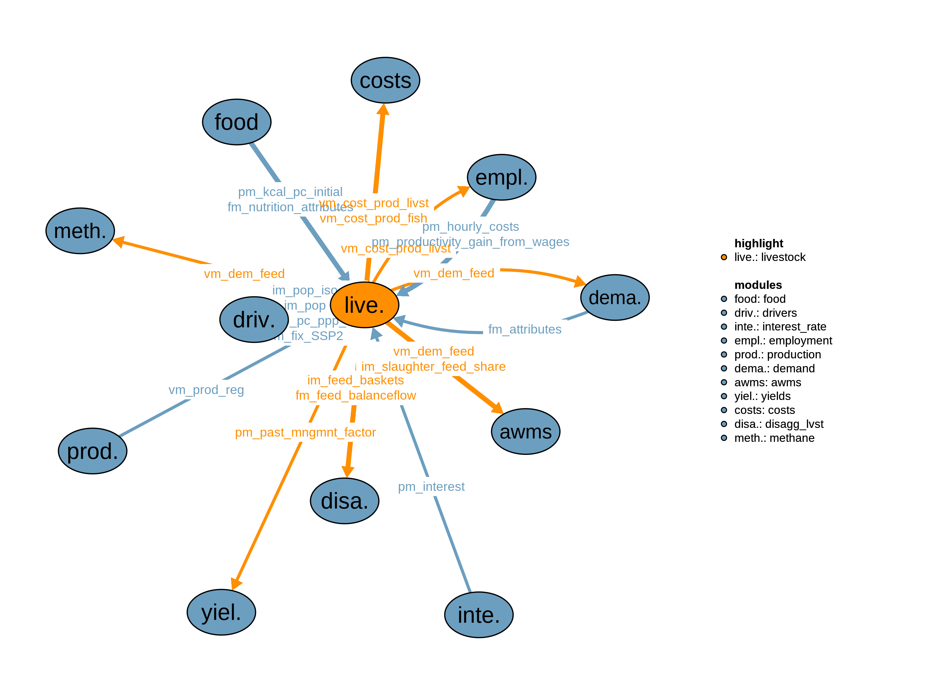
The livestock module calculates how much and what kind of biomass is required as feed to produce livestock food commodities.
For this purpose, the livestock module provides for every time-step
regional and product-specific feed baskets that determine type and
magnitude of feed needed to produce one unit of livestock commodities.
Estimated pasture feed demand is also relevant for the module 31_past in order to derive required pasture
areas. The information flow between the livestock and the pasture module
is organized via interfaces vm_dem_feed,
vm_supply and vm_prod_reg via modules 16_demand and 21_trade. Feed demand estimates are also
required for the modules 53_methane and 55_awms. Additionally, the livestock module
provides production costs for livestock commodities.
| Description | Unit | A | B | |
|---|---|---|---|---|
| fm_attributes (attributes, kall) |
Conversion factors - where X is ton N P K C DM WM or PJ GE | \(X/tDM\) | x | x |
| fm_nutrition_attributes (t_all, kall, nutrition) |
Nutrition attributes of food items dedicated for fooduse | \(10^6 kcal/tDM | t Protein/tDM\) | x | x |
| im_gdp_pc_ppp_iso (t_all, iso) |
Per capita income in purchasing power parity | \(USD_{05PPP}/cap/yr\) | x | x |
| im_pop (t_all, i) |
Population | \(10^6/yr\) | x | x |
| im_pop_iso (t_all, iso) |
Population | \(10^6/yr\) | x | x |
| pm_hourly_costs (t, i, wage_scen) |
Hourly labor costs in agriculture on regional level before and after including wage scenario | \(USD_{MER}05/hour\) | x | x |
| pm_interest (t_all, i) |
Interest rate in each region and timestep | \(\%/yr\) | x | |
| pm_kcal_pc_initial (t, i, kall) |
Per capita consumption in food demand model before price shock | \(kcal/capita/day\) | x | x |
| pm_productivity_gain_from_wages (t, i) |
Multiplicative factor describing productivity gain related to higher wages | \(1\) | x | x |
| sm_fix_SSP2 | year until which all parameters are fixed to SSP2 values | \(year\) | x | x |
| vm_prod_reg (i, kall) |
Regional aggregated production | \(10^6 tDM/yr\) | x | x |
| Description | Unit | |
|---|---|---|
| fm_feed_balanceflow (t_all, i, kap, kall) |
Balanceflow balance difference between estimated feed baskets and FAO | \(10^6 tDM\) |
| im_feed_baskets (t_all, i, kap, kall) |
Feed baskets in tDM per tDM livestock product | \(1\) |
| im_slaughter_feed_share (t_all, i, kap, attributes) |
Share of feed that is incorporated in animal biomass | \(1\) |
| pm_past_mngmnt_factor (t, i) |
Regional pasture management intensification factor | \(1\) |
| vm_cost_prod_fish (i) |
Fish factor costs | \(10^6 USD_{05MER}/yr\) |
| vm_cost_prod_livst (i, factors) |
Livestock factor costs | \(10^6 USD_{05MER}/yr\) |
| vm_dem_feed (i, kap, kall) |
Regional feed demand including byproducts | \(10^6 tDM/yr\) |
The fbask_jan16 realization of the livestock module is based on the
methodology as described in Weindl, Bodirsky, et al. (2017)
and Weindl,
Popp, et al. (2017). An important part of the feed
demand calculations is conducted outside of the core MAgPIE-GAMS code.
Livestock products (ruminant meat, whole-milk, pork, poultry meat and
eggs) are supplied by five animal food systems (beef cattle, dairy
cattle, pigs, broilers and laying hens). The parameterization of the
livestock sector in the initial year is consistent with FAO statistics
regarding livestock production, livestock productivity and concentrate
feed use. The fbask_jan16 realization requires regional and
product-specific feed baskets that are calculated by a set of
preprocessing routines outside of the MAgPIE-GAMS code. Following the
methodology of Wirsenius (2000),
feed conversion (total feed input per product output in dry matter) and
feed baskets (demand for different feed types per product output in dry
matter) are derived by compiling system-specific feed energy balances.
For the establishment of these balances, we apply feed energy
requirements per output, as estimated by wirsenius_human_2000 for each
animal function and animal food system. These estimates are based on
standardized bio-energetic equations and include the minimum energy
requirements for maintenance, growth, lactation, reproduction and other
basic biological functions of the animals. Moreover, they comprise a
general allowance for basic activity and temperature effects. By
distributing the available feed at country level to animal food systems
according to their feed energy demand and dividing resulting dry matter
feed use by the production volume of the respective systems, we obtain
both estimates for feed conversion and feed baskets across different
animal food systems and countries. To facilitate projections of feed
conversion and feed baskets, we create regression models with livestock
productivity (annual production per animal [ton fresh
matter/animal/year]) as predictor, which permit the construction of
livestock feeding scenarios. Currently, feeding scenarios are derived
based on exogenous livestock productivity scenarios consistent with the
storylines of the Shared Socioeconomic Pathways (SSPs). For beef cattle,
pigs and broilers, livestock productivity is defined as meat production
per animals in stock (e.g. total cattle herd) and for dairy cattle and
laying hen as milk or egg production per producing animals (e.g. milk
cows). A power function is used to describe the functional relation
between feed conversion and livestock productivity:  In the case of feed composition, we use an additional proxy parameter in
our analysis. What type of biomass is used to feed animals is to a
certain extent influenced by universal aspects (e.g. the need for more
energy-rich feed at higher productivity levels), whereas other aspects
are strongly influenced by geographical location (e.g. availability and
costs of permanent pasture compared to cropland feed, agro-ecological
and climatic conditions that favour selected feed items; socio-cultural
determinants etc.). For cattle systems the proxy (climate-zone specific
factor) was determined by calculating the share of the national
population living in arid and cold climate zones.
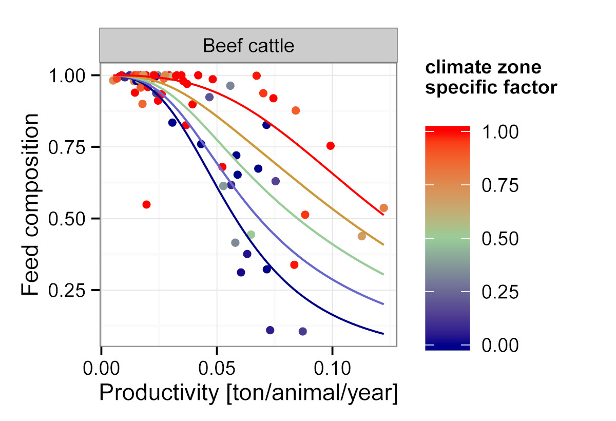
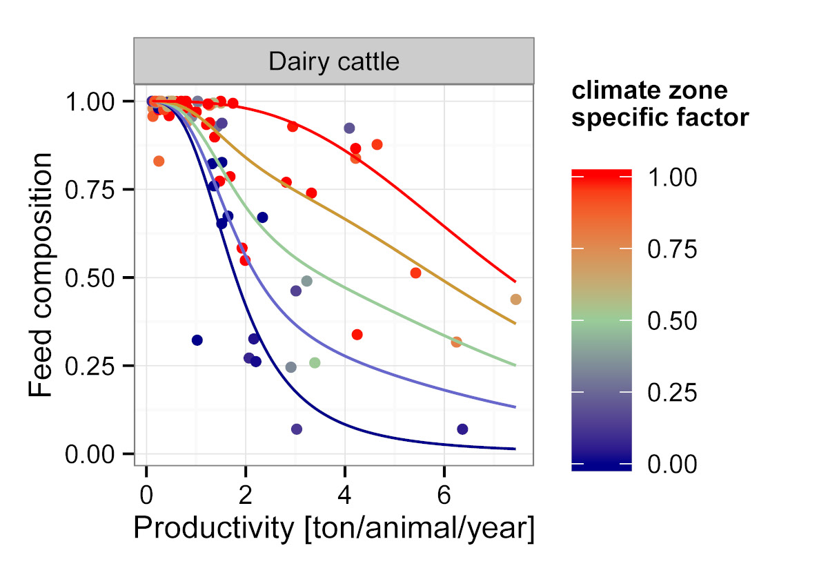 These relationships between feed baskets and livestock productivity are
used to construct feeding scenarios that reflect the narratives of the
SSPs. The resulting feed baskets enter the MAgPIE model as
scenario-dependent input data and are crucial for the feed demand
calculations in the livestock module.
Demand for different feed items is derived by multiplying the
regional livestock production with the respective feed baskets.
Additionally, inconsistencies with the FAO inventory of national feed
use in the case of crops as well as consideration of alternative feed
sources that reduce e.g. the demand for grazed biomass like scavenging
and roadside grazing are balanced out by the parameter
fm_feed_balanceflow.
\[\begin{multline*} vm\_dem\_feed(i2,kap,kall) \geq vm\_prod\_reg(i2,kap) \cdot \sum_{ct}im\_feed\_baskets(ct,i2,kap,kall) +\sum_{ct}fm\_feed\_balanceflow(ct,i2,kap,kall) \end{multline*}\]
Factor requirement costs (e.g. labour, capital, but without costs for
feed) of livestock production depend on the amount of production and the
per-unit costs. For ruminant products (milk and meet), we use a
regression of per-unit factor costs from the GTAP database (Narayanan and
Walmsley 2008) and livestock productivity. Here, factor costs
rise with intensification. The per-unit costs for non-ruminants and fish
are assumed to be independent from productivity trajectories for
simplification. Therefore,
i70_cost_regr(i,kli,"cost_regr_b") is set to zero in the
case of livestock products generated in monogastric systems. To account
for increased hourly labor costs and producitivity in case of an
external wage scenario, the total labor costs are scaled by the
corresponding increase in hourly labor costs and the related
productivity gain from 36_employment.
\[\begin{multline*} vm\_cost\_prod\_livst(i2,"labor") = \sum_{kli}\left( vm\_prod\_reg(i2,kli) \cdot \sum_{ct} i70\_fac\_req\_livst(ct,i2,kli)\right) \cdot \sum_{ct} p70\_cost\_share\_livst(ct,i2,"labor") \cdot \sum_{ct}\left( \left(\frac{1}{pm\_productivity\_gain\_from\_wages(ct,i2)}\right) \cdot \left(\frac{pm\_hourly\_costs(ct,i2,"scenario") }{ pm\_hourly\_costs(ct,i2,"baseline")}\right)\right) \end{multline*}\]
\[\begin{multline*} vm\_cost\_prod\_livst(i2,"capital") = \sum_{kli}\left( vm\_prod\_reg(i2,kli) \cdot \sum_{ct} i70\_fac\_req\_livst(ct,i2,kli)\right) \cdot \sum_{ct} p70\_cost\_share\_livst(ct,i2,"capital") \end{multline*}\]
\[\begin{multline*} vm\_cost\_prod\_fish(i2) = vm\_prod\_reg(i2,"fish") \cdot i70\_cost\_regr(i2,"fish","cost\_regr\_a") \end{multline*}\]
The fbask_jan16 realization of the livestock module also estimates an
exogenous pasture management factor pm_past_mngmnt_factor
that is used to scale biophysical pasture yields in the module 14_yields. The exogenous calculation of pasture
management requires information on changes in the number of cattle
reared to fulfil the food demand for ruminant livestock products:
p70_cattle_stock_proxy(t,i) = im_pop(t,i)*pm_kcal_pc_initial(t,i,"livst_rum")
                  /i70_livestock_productivity(t,i,"sys_beef");
p70_milk_cow_proxy(t,i) = im_pop(t,i)*pm_kcal_pc_initial(t,i,"livst_milk")
                  /i70_livestock_productivity(t,i,"sys_dairy");
The lower bound for p70_cattle_stock_proxy and
p70_milk_cow_proxy is set to 20% of initial values in
1995:
p70_cattle_stock_proxy(t,i)$(p70_cattle_stock_proxy(t,i) < 0.2*p70_cattle_stock_proxy("y1995",i)) = 0.2*p70_cattle_stock_proxy("y1995",i);
p70_milk_cow_proxy(t,i)$(p70_milk_cow_proxy(t,i) < 0.2*p70_milk_cow_proxy("y1995",i)) = 0.2*p70_milk_cow_proxy("y1995",i);
The parameter p70_cattle_feed_pc_proxy is a proxy for
regional daily per capita feed demand for pasture biomass driven by
demand for beef and dairy products, which is later used for weighted
aggregation.
p70_cattle_feed_pc_proxy(t,i,kli_rd) = pm_kcal_pc_initial(t,i,kli_rd)*im_feed_baskets(t,i,kli_rd,"pasture")/(fm_nutrition_attributes(t,kli_rd,"kcal") * 10**6);The parameter p70_incr_cattle describes the changes in
the number of cattle relative to the previous time step:
if (ord(t)>1,
   p70_incr_cattle(t,i) = ( (p70_cattle_feed_pc_proxy(t,i,"livst_rum")  + 10**(-6))* (p70_cattle_stock_proxy(t,i)/p70_cattle_stock_proxy(t-1,i))
                                          +  (p70_cattle_feed_pc_proxy(t,i,"livst_milk") + 10**(-6)) * (p70_milk_cow_proxy(t,i)/p70_milk_cow_proxy(t-1,i)) )
                                        / sum(kli_rd, p70_cattle_feed_pc_proxy(t,i,kli_rd) + 10**(-6));
else
   p70_incr_cattle(t,i) = 1;
);
The pasture management factor is calculated by applying a linear relationship that links changes in pasture management with changes in the number of cattle:
if (m_year(t) <= s70_past_mngmnt_factor_fix,
   pm_past_mngmnt_factor(t,i) = 1;
else
   pm_past_mngmnt_factor(t,i) =   ( (s70_pyld_intercept + f70_pyld_slope_reg(i)*p70_incr_cattle(t,i)**(5/(m_year(t)-m_year(t-1)))
           )**((m_year(t)-m_year(t-1))/5) )*pm_past_mngmnt_factor(t-1,i);
 );
Limitations Intensification of livestock production and related changes in livestock feeding are modelled exogenously. Therefore, the livestock sector does not endogenously respond to demand and climate shocks and policies, e.g. targeting climate protection.
The fbask_jan16_sticky realization of the livestock module is based
on the fbask_jan16 realization, and only differs from it by implementing
capital stocks as introduced in the sticky_feb18 factor
cost module realization.
The methodology of fbask_jan16 is described in Weindl, Bodirsky, et al. (2017)
and Weindl,
Popp, et al. (2017). An important part of the feed
demand calculations is conducted outside of the core MAgPIE-GAMS code.
Livestock products (ruminant meat, whole-milk, pork, poultry meat and
eggs) are supplied by five animal food systems (beef cattle, dairy
cattle, pigs, broilers and laying hens). The parameterization of the
livestock sector in the initial year is consistent with FAO statistics
regarding livestock production, livestock productivity and concentrate
feed use. The fbask_jan16 realization requires regional and
product-specific feed baskets that are calculated by a set of
preprocessing routines outside of the MAgPIE-GAMS code. Following the
methodology of Wirsenius (2000),
feed conversion (total feed input per product output in dry matter) and
feed baskets (demand for different feed types per product output in dry
matter) are derived by compiling system-specific feed energy balances.
For the establishment of these balances, we apply feed energy
requirements per output, as estimated by wirsenius_human_2000 for each
animal function and animal food system. These estimates are based on
standardized bio-energetic equations and include the minimum energy
requirements for maintenance, growth, lactation, reproduction and other
basic biological functions of the animals. Moreover, they comprise a
general allowance for basic activity and temperature effects. By
distributing the available feed at country level to animal food systems
according to their feed energy demand and dividing resulting dry matter
feed use by the production volume of the respective systems, we obtain
both estimates for feed conversion and feed baskets across different
animal food systems and countries. To facilitate projections of feed
conversion and feed baskets, we create regression models with livestock
productivity (annual production per animal [ton fresh
matter/animal/year]) as predictor, which permit the construction of
livestock feeding scenarios. Currently, feeding scenarios are derived
based on exogenous livestock productivity scenarios consistent with the
storylines of the Shared Socioeconomic Pathways (SSPs). For beef cattle,
pigs and broilers, livestock productivity is defined as meat production
per animals in stock (e.g. total cattle herd) and for dairy cattle and
laying hen as milk or egg production per producing animals (e.g. milk
cows). A power function is used to describe the functional relation
between feed conversion and livestock productivity:  In the case of feed composition, we use an additional proxy parameter in
our analysis. What type of biomass is used to feed animals is to a
certain extent influenced by universal aspects (e.g. the need for more
energy-rich feed at higher productivity levels), whereas other aspects
are strongly influenced by geographical location (e.g. availability and
costs of permanent pasture compared to cropland feed, agro-ecological
and climatic conditions that favour selected feed items; socio-cultural
determinants etc.). For cattle systems the proxy (climate-zone specific
factor) was determined by calculating the share of the national
population living in arid and cold climate zones.
 These relationships between feed baskets and livestock productivity are
used to construct feeding scenarios that reflect the narratives of the
SSPs. The resulting feed baskets enter the MAgPIE model as
scenario-dependent input data and are crucial for the feed demand
calculations in the livestock module.
In this realization the capital share of livestock production cost
does not have to be paid every timestep, but is fulfilled by having a
corresponding capital stock, which mostly persists across timesteps.
(See s70_depreciation_rate) This means that the production
becomes cheaper in regions with higher capital shares and existing
corresponding capital stocks, which makes the livestock production
“stick” to some degree to existing levels. Another effect is that
production increases are more likely to occur in regions of more capital
intensive livestock systems with already established stocks.
The realization is based on the sticky_feb18 factor cost
realization, but also differs from it in some ways. At the creation time
the main differences were: 1. capital stocks are on the regional level
not on cluster level 2. no differentiation of mobile and immobile
capital - all capital stocks are immobile
Demand for different feed items is derived by multiplying the
regional livestock production with the respective feed baskets.
Additionally, inconsistencies with the FAO inventory of national feed
use in the case of crops as well as consideration of alternative feed
sources that reduce e.g. the demand for grazed biomass like scavenging
and roadside grazing are balanced out by the parameter
fm_feed_balanceflow.
\[\begin{multline*} vm\_dem\_feed(i2,kap,kall) \geq vm\_prod\_reg(i2,kap) \cdot \sum_{ct}im\_feed\_baskets(ct,i2,kap,kall) +\sum_{ct}fm\_feed\_balanceflow(ct,i2,kap,kall) \end{multline*}\]
Factor requirement costs (e.g. labour, capital, but without costs for
feed) of livestock production depend on the amount of production and the
per-unit costs. For ruminant products (milk and meet), we use a
regression of per-unit factor costs from the GTAP database (Narayanan and
Walmsley 2008) and livestock productivity. Here, factor costs
rise with intensification. The per-unit costs for non-ruminants and fish
are assumed to be independent from productivity trajectories for
simplification. Therefore,
i70_cost_regr(i,kli,"cost_regr_b") is set to zero in the
case of livestock products generated in monogastric systems. To account
for increased hourly labor costs and producitivity in case of an
external wage scenario, the total labor costs are scaled by the
corresponding increase in hourly labor costs and the related
productivity gain from 36_employment.
\[\begin{multline*} vm\_cost\_prod\_livst(i2,"labor") = \sum_{kli}\left( vm\_prod\_reg(i2,kli) \cdot \sum_{ct} i70\_fac\_req\_livst(ct,i2,kli)\right) \cdot \sum_{ct} p70\_cost\_share\_livst(ct,i2,"labor") \cdot \sum_{ct}\left( \left(\frac{1}{pm\_productivity\_gain\_from\_wages(ct,i2)}\right) \cdot \left(\frac{pm\_hourly\_costs(ct,i2,"scenario") }{ pm\_hourly\_costs(ct,i2,"baseline")}\right)\right) \end{multline*}\]
\[\begin{multline*} vm\_cost\_prod\_fish(i2) = vm\_prod\_reg(i2,"fish") \cdot i70\_cost\_regr(i2,"fish","cost\_regr\_a") \end{multline*}\]
Investment costs are calculated analogously to the
sticky_feb18 realization. The costs are annuitized, and
corrected to make sure that the annual depreciation of the current
time-step is accounted for.
\[\begin{multline*} vm\_cost\_prod\_livst(i2,"capital") = \sum_{kli}v70\_investment(i2,kli) \cdot \left(\left(1-s70\_depreciation\_rate\right) \cdot \sum_{ct}\left(\frac{pm\_interest(ct,i2)}{\left(1+pm\_interest(ct,i2)\right)}\right) + s70\_depreciation\_rate\right) \end{multline*}\]
Each livestock activity requires a certain capital stock that depends on the production. The following equations make sure that new land expansion is equipped with capital stock, and that depreciation of pre-existing capital is replaced.
\[\begin{multline*} v70\_investment(i2,kli) \geq vm\_prod\_reg(i2,kli) \cdot \sum_{ct} p70\_capital\_need(ct,i2,kli) - \sum_{ct} p70\_capital(ct,i2,kli) \end{multline*}\]
This realization of the livestock module also estimates an exogenous
pasture management factor pm_past_mngmnt_factor that is
used to scale biophysical pasture yields in the module 14_yields. The exogenous calculation of pasture
management requires information on changes in the number of cattle
reared to fulfil the food demand for ruminant livestock products:
p70_cattle_stock_proxy(t,i) = im_pop(t,i)*pm_kcal_pc_initial(t,i,"livst_rum")
                  /i70_livestock_productivity(t,i,"sys_beef");
p70_milk_cow_proxy(t,i) = im_pop(t,i)*pm_kcal_pc_initial(t,i,"livst_milk")
                  /i70_livestock_productivity(t,i,"sys_dairy");
The lower bound for p70_cattle_stock_proxy and
p70_milk_cow_proxy is set to 20% of initial values in
1995:
p70_cattle_stock_proxy(t,i)$(p70_cattle_stock_proxy(t,i) < 0.2*p70_cattle_stock_proxy("y1995",i)) = 0.2*p70_cattle_stock_proxy("y1995",i);
p70_milk_cow_proxy(t,i)$(p70_milk_cow_proxy(t,i) < 0.2*p70_milk_cow_proxy("y1995",i)) = 0.2*p70_milk_cow_proxy("y1995",i);
The parameter p70_cattle_feed_pc_proxy is a proxy for
regional daily per capita feed demand for pasture biomass driven by
demand for beef and dairy products, which is later used for weighted
aggregation.
p70_cattle_feed_pc_proxy(t,i,kli_rd) = pm_kcal_pc_initial(t,i,kli_rd)*im_feed_baskets(t,i,kli_rd,"pasture")/(fm_nutrition_attributes(t,kli_rd,"kcal") * 10**6);The parameter p70_incr_cattle describes the changes in
the number of cattle relative to the previous time step:
if (ord(t)>1,
   p70_incr_cattle(t,i) = ( (p70_cattle_feed_pc_proxy(t,i,"livst_rum")  + 10**(-6))* (p70_cattle_stock_proxy(t,i)/p70_cattle_stock_proxy(t-1,i))
                                          +  (p70_cattle_feed_pc_proxy(t,i,"livst_milk") + 10**(-6)) * (p70_milk_cow_proxy(t,i)/p70_milk_cow_proxy(t-1,i)) )
                                        / sum(kli_rd, p70_cattle_feed_pc_proxy(t,i,kli_rd) + 10**(-6));
else
   p70_incr_cattle(t,i) = 1;
);
The pasture management factor is calculated by applying a linear relationship that links changes in pasture management with changes in the number of cattle:
if (m_year(t) <= s70_past_mngmnt_factor_fix,
   pm_past_mngmnt_factor(t,i) = 1;
else
   pm_past_mngmnt_factor(t,i) =   ( (s70_pyld_intercept + f70_pyld_slope_reg(i)*p70_incr_cattle(t,i)**(5/(m_year(t)-m_year(t-1)))
           )**((m_year(t)-m_year(t-1))/5) )*pm_past_mngmnt_factor(t-1,i);
 );
Capital update from the last investment
Limitations Intensification of livestock production and related changes in livestock feeding are modelled exogenously. Therefore, the livestock sector does not endogenously respond to demand and climate shocks and policies, e.g. targeting climate protection.
| Description | Unit | A | B | |
|---|---|---|---|---|
| f70_cap_share_reg (share_regr) |
Parameters for regression | x | x | |
| f70_cost_regr (kap, cost_regr) |
Factor requirements livestock (USD04 per tDM (A) and USD | \(B)\) | x | x |
| f70_feed_baskets (t_all, i, kap, kall, feed_scen70) |
Feed baskets in tDM per tDM livestock product | \(1\) | x | x |
| f70_hist_cap_share (t_all, i) |
Historical capital share | x | x | |
| f70_hist_factor_costs_livst (t_all, i, kli) |
Historical factor costs in livestock production | \(10^6 USD_{05MER}\) | x | x |
| f70_hist_prod_livst (t_all, i, kli, attributes) |
Historical production quantity of livestock products | \(10^6 t\) | x | x |
| f70_livestock_productivity (t_all, i, sys, feed_scen70) |
Productivity indicator for livestock production | \(t FM/animal\) | x | x |
| f70_pyld_slope_reg (i) |
Regional slope of linear relationship determining pasture intensification | \(1\) | x | x |
| f70_slaughter_feed_share (t_all, i, kap, attributes, feed_scen70) |
Share of feed that is incorprated in animal biomass | \(1\) | x | x |
| i70_cereal_scp_fadeout (t_all, i) |
Cereal feed fadeout (share 0-1) to be replaced by SCP | \(1\) | x | x |
| i70_cost_regr (i, kap, cost_regr) |
Regression coefficients for livestock factor requirements | \(1\) | x | x |
| i70_fac_req_livst (t_all, i, kli) |
Factor requirements | \(USD_{05MER}/tDM\) | x | x |
| i70_foddr_scp_fadeout (t_all, i) |
Fodder fadeout (share 0-1) to be replaced by SCP | \(1\) | x | x |
| i70_livestock_productivity (t_all, i, sys) |
Productivity indicator for livestock production | \(t FM/animal/yr\) | x | x |
| p70_capital (t, i, kli) |
Preexisting immobile capital stocks before investment | \(10^6 USD_{05MER}\) | x | |
| p70_capital_need (t, i, kli) |
Capital requirements per unit of output | \(USD_{05MER}/ton DM\) | x | |
| p70_cattle_feed_pc_proxy (t, i, kli_rd) |
Proxy for daily per capita feed demand for pasture biomass driven by demand for beef and dairy products | \(tDM/capita/day\) | x | x |
| p70_cattle_stock_proxy (t, i) |
Proxy for cattle stocks needed to fullfil food demand for ruminant meat | \(10^6 animals/yr\) | x | x |
| p70_cereal_subst_fader (t_all) |
Cereal feed substitution with SCP fader | \(1\) | x | x |
| p70_cost_share_calibration (i) |
Summation factor used to calibrate calculated capital shares with historical values | \(1\) | x | x |
| p70_cost_share_livst (t, i, factors) |
Capital and labor shares of the regional factor costs for plant production for livestock | \(1\) | x | x |
| p70_country_dummy (iso) |
Dummy parameter indicating whether country is affected by feed scenarios | \(1\) | x | x |
| p70_feedscen_region_shr (t_all, i) |
Weighted share of region with regards to feed scenario of countries | \(1\) | x | x |
| p70_foddr_subst_fader (t_all) |
Foddr substitution with SCP fader | \(1\) | x | x |
| p70_incr_cattle (t, i) |
Change in estimated cattle stocks attributed to food demand projections | \(1\) | x | x |
| p70_initial_1995_prod (i, kli) |
Initial regional production of livestock products taken from 1995 | \(10^6 ton DM\) | x | |
| p70_milk_cow_proxy (t, i) |
Proxy for milk cows needed to fullfil food demand for milk | \(10^6 animals/yr\) | x | x |
| q70_cost_prod_fish (i) |
Regional factor input costs for fish production | x | x | |
| q70_cost_prod_liv_capital (i) |
Regional capital costs for livestock production | x | x | |
| q70_cost_prod_liv_labor (i) |
Regional labor costs for livestock production | x | x | |
| q70_feed (i, kap, kall) |
Regional feed demand | x | x | |
| q70_investment (i, kli) |
Regional investments into farm capital | x | ||
| s70_cereal_scp_substitution | Cereal feed substitution with SCP share | \(1\) | x | x |
| s70_depreciation_rate | Yearly depreciation rate for capital stocks | x | ||
| s70_feed_substitution_start | Feed substitution start year | x | x | |
| s70_feed_substitution_target | Feed substitution target year | x | x | |
| s70_foddr_scp_substitution | Fodder substitution with SCP share | \(1\) | x | x |
| s70_multiplicator_capital_need | Multiplicator for capital need in livestock production | x | ||
| s70_past_mngmnt_factor_fix | Year until the pasture management factor is fixed to 1 | x | x | |
| s70_pyld_intercept | Intercept of linear relationship determining pasture intensification | \(1\) | x | x |
| s70_subst_functional_form | Switch for functional form of feed substitution scenario fader | \(1\) | x | x |
| v70_investment (i, kli) |
Investment in immobile farm capital | \(10^6 USD_{05MER}/yr\) | x |
| description | |
|---|---|
| attributes | Product attributes characterizing a product (such as weight or energy content) |
| cost_regr | Cost regression parameters |
| ct(t) | Current time period |
| factors | factors included in factor requirements |
| fadeoutscen70 | Feed substitution scenarios including functional forms with targets and transition periods |
| feed_scen70 | scenarios |
| i | all economic regions |
| i_to_iso(i, iso) | mapping regions to iso countries |
| i2(i) | World regions (dynamic set) |
| iso | list of iso countries |
| kall | All products in the sectoral version |
| kap(k) | Animal products |
| kcer70(kall) | Cereals |
| kli_rd(kap) | Ruminant meat and dairy products |
| kli(kap) | Livestock products |
| nutrition | Nutrition attributes |
| reg | regression parameters for capital calculation |
| scen_countries70(iso) | countries to be affected by selected feed sceanrio |
| share_regr | regression parameters for capital share calculation |
| sys | Livestock production systems |
| sys_meat(sys) | Livestock meat production systems |
| sys_nonmeat(sys) | Livestock non-meat production systems |
| sys_to_kli(sys, kli) | Mapping between livestock producton systems and livestock products |
| t_all(t_ext) | 5-year time periods |
| t_past(t_all) | Timesteps with observed data |
| t(t_all) | Simulated time periods |
| type | GAMS variable attribute used for the output |
| wage_scen | version of wages |
Isabelle Weindl, Benjamin Bodirsky
09_drivers, 11_costs, 12_interest_rate, 14_yields, 15_food, 16_demand, 17_production, 36_employment, 53_methane, 55_awms, 71_disagg_lvst