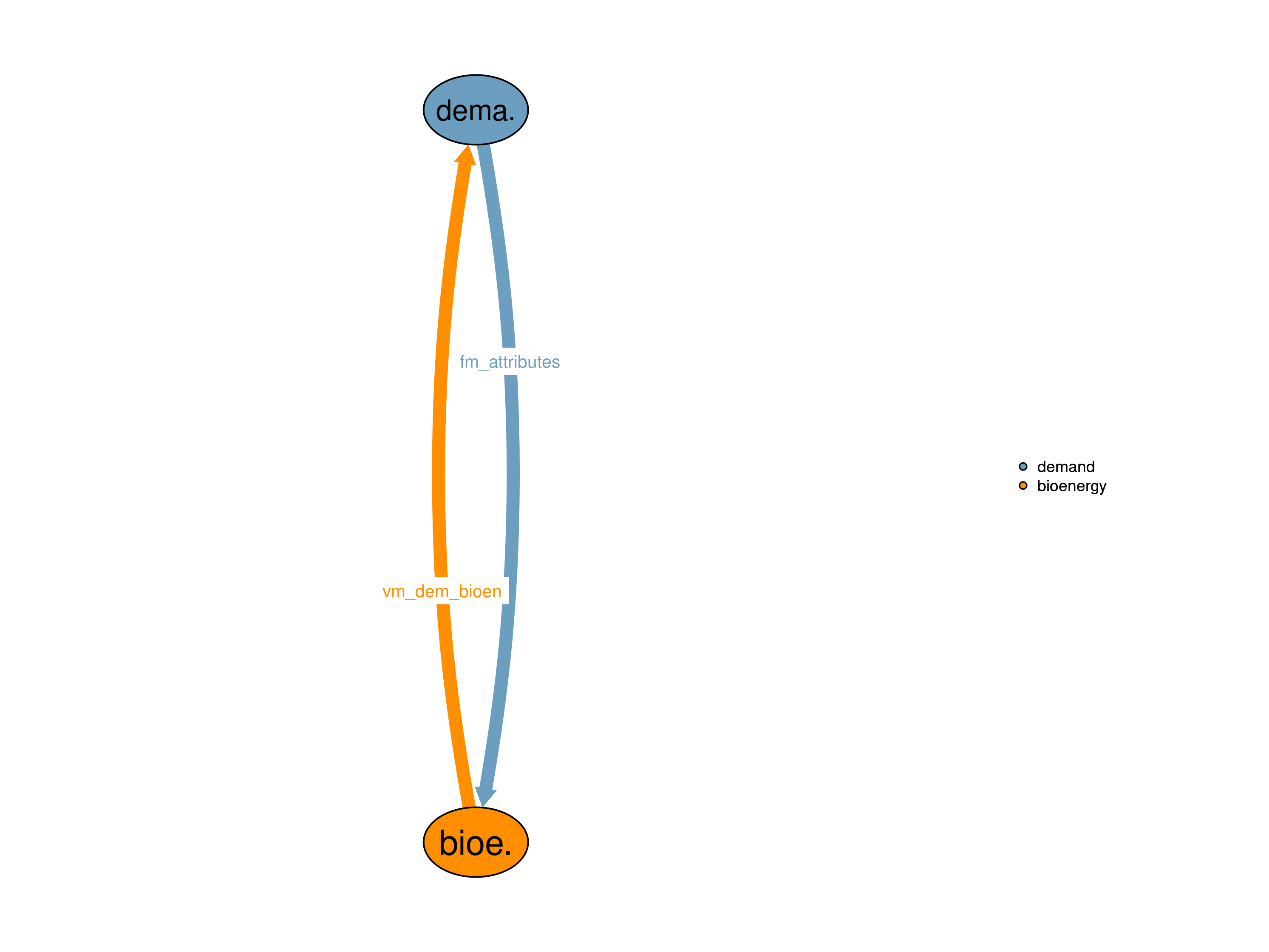
The bioenergy module provides a regional and crop-specific bioenergy demand \(vm\_dem\_bioen\) to the model (to the 16_demand module). For this calculation it requires information on gross energy content (provided by 16_demand module).
In addition to calculation of bioenergy quantities, the costs associated with the production are provided to the objective function in the 11_costs module.
| Description | Unit | A | |
|---|---|---|---|
| fm_attributes (attributes, kall) |
Conversion factors - where X is ton N P K C DM WM or PJ GE | \(X/tDM\) | x |
| Description | Unit | |
|---|---|---|
| vm_dem_bioen (i, kall) |
Regional bioenergy demand | \(10^6 tDM/yr\) |
Calculation of first and second generation bioenergy demand on the regional level.
The bioenergy demand calculation for second generation bioenergy is based on the following two equations from which always only one is active: If \(c60\_biodem\_level\) is 1 (regional) the right hand side of the first equation is set to 0, if it is 0 (global) the right hand side of the second equation is set to 0.
\[\begin{multline*} \sum_{kbe60,i2}\left( vm\_dem\_bioen(i2,kbe60) \cdot fm\_attributes("ge",kbe60)\right) \geq \sum_{ct,i2}i60\_bioenergy\_dem(ct,i2) \cdot \left(1-c60\_biodem\_level\right) \end{multline*}\]
\[\begin{multline*} \sum_{kbe60}\left( vm\_dem\_bioen(i2,kbe60) \cdot fm\_attributes("ge",kbe60)\right) \geq \sum_{ct}i60\_bioenergy\_dem(ct,i2) \cdot c60\_biodem\_level \end{multline*}\]
Except the implementation of the switches and the fact that in the first equation the bioenergy demand is summed up to a global demand both equations act the same way: In both cases the equation just makes sure that the sum over all second generation energy crop of the bioenergy demand is greater or equal to the demand actually given by the input file \(i60\_bioenergy\_dem\).
\[\begin{multline*} \sum_{kres}\left( vm\_dem\_bioen(i2,kres) \cdot fm\_attributes("ge",kres) - \sum_{ct}\left(f60\_1stgen\_bioenergy\_dem\left(ct,i2,"\%c60\_1stgen\_biodem\%",kres\right)\right)\right) \geq \sum_{ct}i60\_res\_2ndgenBE\_dem(ct,i2) \end{multline*}\]
There is additionally some demand of residues for second generation bioenergy \(i60\_res\_2ndgenBE\_dem\), which is exogenously provided by the estimation that roughly 33% of available residues for recycling on cropland can be used for 2nd generation bioenergy depending on the SSP scenario, since residue stock and use is mainly driven by population and GDP.
For first generation bioenergy, input is provided on regional level fixing the bioenergy demand variable \(vm\_dem\_bioen\) to the input values \(f60\_dem\_1stgen\_bioen\) (in presolve.gms).
vm_dem_bioen.fx(i,kall) = f60_1stgen_bioenergy_dem(t,i,"%c60_1stgen_biodem%",kall)
                          /fm_attributes("ge",kall);
The used first generation bioenergy trajectory contains demand until 2050 based on currently established and planned bioenergy policies (Lotze-Campen et al. (2014)). For the time after 2050 it is assumed that bioenergy production will be fully transformed to 2nd generation bioenergy crops and residues because of their higher estimated efficiency respectively their low costs.
For second generation bioenergy (kbe60 = bioenergy grasses and bioenergy trees), input is given either on regional or global level (defined via switch \(c60\_biodem\_level\)). As the bioenergy demand for all crop types was fixed in the first step it now has to be released again for second generation bioenergy crops (kbe60).
vm_dem_bioen.up(i,kbe60) = Inf;
vm_dem_bioen.lo(i,kbe60) = 0;
Relax the upper bound for residues.
vm_dem_bioen.up(i,kres) = Inf;Limitations There are no known limitations.
| Description | Unit | A | |
|---|---|---|---|
| c60_biodem_level | bioenergy demand level indicator 1 for regional and 0 for global demand | \(1\) | x |
| f60_1stgen_bioenergy_dem (t_all, i, scen1st60, kall) |
annual 1st generation bioenergy demand | \(10^6 GJ/yr\) | x |
| f60_bioenergy_dem (t_all, i, scen2nd60) |
annual bioenergy demand (regional) | \(10^6 GJ/yr\) | x |
| f60_res_2ndgenBE_dem (t_all, i, scen2ndres60) |
annual residue demand for 2nd generation bioenergy(regional) | \(10^6 GJ/yr\) | x |
| i60_bioenergy_dem (t, i) |
Regional bioenergy demand per year | \(10^6 GJ/yr\) | x |
| i60_res_2ndgenBE_dem (t, i) |
Regional residue demand for 2nd generation bioenergy per year | \(10^6 GJ/yr\) | x |
| q60_bioenergy_glo | Global bioenergy demand | \(10^6 GJ/yr\) | x |
| q60_bioenergy_reg (i) |
Regional bioenergy demand | \(10^6 GJ/yr\) | x |
| q60_res_2ndgenBE (i) |
Regional residue demand for 2nd generation bioenergy | \(10^6 GJ/yr\) | x |
| description | |
|---|---|
| attributes | Product attributes characterizing a product (such as weight or energy content) |
| ct(t) | Current time period |
| i | World regions |
| i2(i) | World regions (dynamic set) |
| kall | All products in the sectoral version |
| kbe60(kcr) | bio energy activities |
| kcr(kve) | Cropping activities |
| kres(kall) | Residues |
| scen1st60 | first generation bioenergy scenarios |
| scen2nd60 | second generation bioenergy scenarios |
| scen2ndres60 | residues for second generation bioenergy scenarios |
| t_all | 5-year time periods |
| t(t_all) | Simulated time periods |
| type | GAMS variable attribute used for the output |
Jan Philipp Dietrich
Lotze-Campen, Hermann, Martin von Lampe, Page Kyle, Shinichiro Fujimori, Petr Havlik, Hans van Meijl, Tomoko Hasegawa, et al. 2014. “Impacts of Increased Bioenergy Demand on Global Food Markets: An AgMIP Economic Model Intercomparison.” Agricultural Economics 45 (1): 103–16. https://doi.org/10.1111/agec.12092.