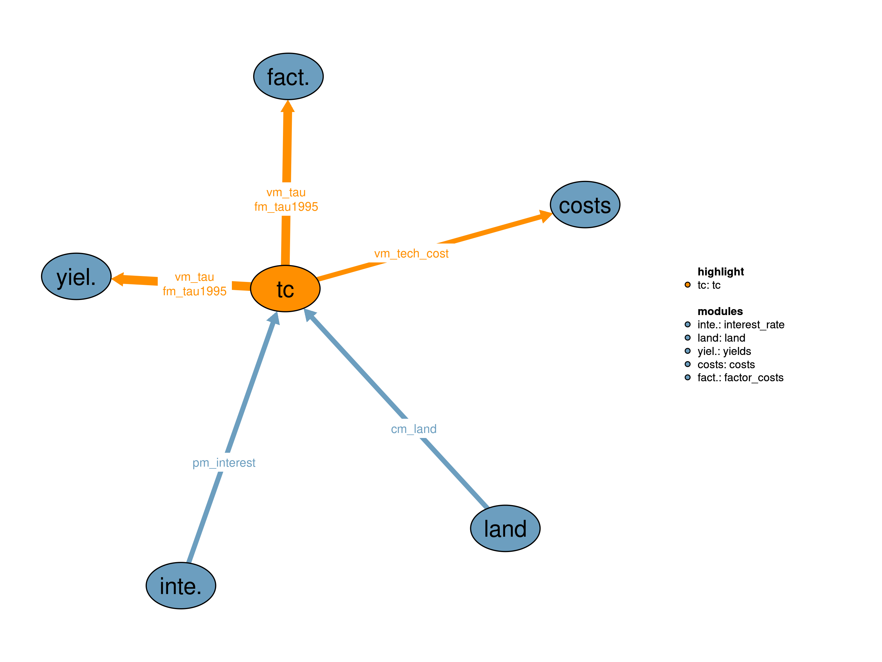
The technological change (TC) module describes the relation between agricultural land use intensity represented by the \(\tau\) factor and the costs which have to be paid for further intensification (technological change costs). Besides cropland expansion (39_landconversion) and trade (21_trade), it describes the third major option of the model to increase regional supply. In order to calculate this relation, the module needs to receive information about the assumed interest rate and assumed investment horizon currently provided by module 12_interest_rate.
Calculated \(\tau\) factors are then used for yields calculation by 14_yields and by 38_factor_costs for the calculation of factor costs.
| Description | Unit | A | |
|---|---|---|---|
| pcm_land (j, land) |
Land area in previous time step | \(10^6 ha\) | x |
| pm_interest (i) |
Current interest rate in each region | \(\%/yr\) | x |
| Description | Unit | |
|---|---|---|
| fm_tau1995 (i) |
Agricultural land use intensity tau in 1995 | \(1\) |
| vm_tau (i) |
Agricultural land use intensity tau | \(1\) |
| vm_tech_cost (i) |
Costs of TC | \(10^6 USD_{05PPP}/yr\) |
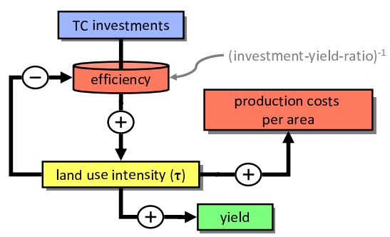
The endo realization stands for endogenous implementation of technological change and land use intensification. The intensification rates are calculated endogenously based on an interplay between land use intensity \(\tau\) and technological change costs (as shown schematically in the figure below). This module realization contains the implementation as described in Dietrich et al. (2014) with two minor modifications:
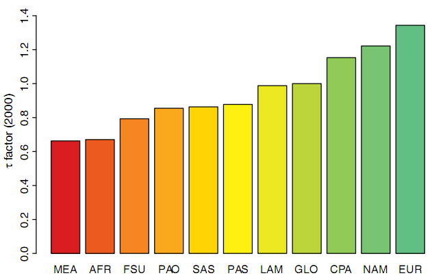
Initial land use intensity \(\tau\) values for the year 2000 come from Dietrich et al. (2012) and are shown below.
Investments into technological change (TC) trigger land use intensification (\(\tau\)) which triggers in turn yields increases. How much intensification can be triggered by an investment, depends on the investment-yield ratio, which in turn depends on the current agricultural land use intensity. The higher the current intensity level, the more expensive the additional intensification will become. The interaction between land use intensity and production costs per area as shown in the schematic is not covered by this module and can be found instead in 38_factor_costs.
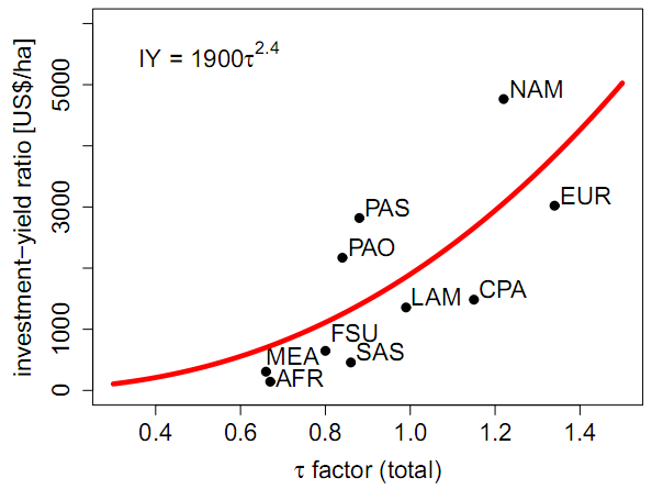
Relative technological change costs v13_cost_tc are calculated as a heuristically derived power function of the land use intensity vm_tau for the investment-yield-ratio (see figure above) multiplied by the current regional crop areas pc13_land (taken from previous time step) and shifted 15 years into the future using the region specific interest rate pm_interest:
\[\begin{multline*} v13\_cost\_tc(i2) = \sum_{ct}\left( pc13\_land(i2) \cdot i13\_tc\_factor(ct,i2) \cdot vm\_tau(i2)^{i13\_tc\_exponent(ct,i2) } \cdot \left(1+pm\_interest(i2)\right)^{15}\right) \end{multline*}\]
The shifting is performed because investments into technological change require on average 15 years of research before a yield increase is achieved, but the model has to see costs and benefits concurrently in order to take the right investment decisions (see also Dietrich et al. (2014)). Investment costs are scaled in relation to crop area, since a wider areal coverage means typically also higher variety in biophysical conditions, which would require more research for the same overall intensity boost.
In order to get the full investments required for the desired intensification the relative technological change costs are multiplied with the given intensification rate. These full costs are then distributed over an infinite time horizon by multiplication with the interest rate pm_interest(i) (annuity with infinite time horizon):
\[\begin{multline*} v13\_tech\_cost\_annuity(i2) = \left(\frac{vm\_tau(i2)}{pc13\_tau(i2)}-1\right) \cdot v13\_cost\_tc(i2) \cdot \frac{ pm\_interest(i2)}{\left(1+pm\_interest(i2)\right)} \end{multline*}\]
Additionally, the technological change costs coming from past investment decisions are added to the technological change costs of the current period:
\[\begin{multline*} vm\_tech\_cost(i2) = v13\_tech\_cost\_annuity(i2) + pc13\_tech\_cost\_past(i2) \end{multline*}\]
Limitations This module significantly reduces the overall computational performance of the model since these endogenous calculations are highly computational intensive.
| Description | Unit | A | |
|---|---|---|---|
| f13_tc_exponent (t_all, scen13) |
Regression exponent | \(1\) | x |
| f13_tc_factor (t_all, scen13) |
Regression factor | \(USD_{05PPP}/ha\) | x |
| f13_tcguess (i) |
Guess for initial annual TC rates | \(1\) | x |
| i13_tc_exponent (t, i) |
Regression exponent | \(1\) | x |
| i13_tc_factor (t, i) |
Regression factor | \(USD_{05PPP}/ha\) | x |
| p13_tech_cost_past (t, i) |
Costs for TC from past | \(10^6 USD_{05PPP}/yr\) | x |
| pc13_land (i) |
Crop land area per region | \(10^6 ha\) | x |
| pc13_tau (i) |
Tau factor of the previous time step | \(1\) | x |
| pc13_tcguess (i) |
Guess for annual tc rates in the next time step | \(1\) | x |
| pc13_tech_cost_past (i) |
Current costs for TC from past | \(10^6 USD_{05PPP}/yr\) | x |
| q13_cost_tc (i) |
Costs for TC | \(10^6 USD_{05PPP}/yr\) | x |
| q13_tech_cost (i) |
Total costs for TC | \(10^6 USD_{05PPP}\) | x |
| q13_tech_cost_annuity (i) |
Annuity costs for TC | \(10^6 USD_{05PPP}/yr\) | x |
| v13_cost_tc (i) |
Technical change costs per region | \(10^6 USD_{05PPP}\) | x |
| v13_tech_cost_annuity (i) |
Annuity costs of TC | \(10^6 USD_{05PPP}/yr\) | x |
| description | |
|---|---|
| cell(i, j) | Mapping between regions i and clusters j |
| ct(t) | Current time period |
| dev | Economic development status |
| i | World regions |
| i2(i) | World regions (dynamic set) |
| j | Spatial clusters |
| land | Land pools |
| scen13 | tc cost scenario |
| scen13_to_dev(scen13, dev) | mapping between tc cost scenarios and development stages |
| t_all | 5-year time periods |
| t_to_i_to_dev(t, i, dev) | Mapping between time region and economic development status |
| t(t_all) | Simulated time periods |
| type | GAMS variable attribute used for the output |
Jan Philipp Dietrich, Christoph Schmitz, Benjamin Bodirsky
10_land, 11_costs, 12_interest_rate, 14_yields, 38_factor_costs
Dietrich, Jan Philipp, Christoph Schmitz, Hermann Lotze-Campen, Alexander Popp, and Christoph Müller. 2014. “Forecasting Technological Change in Agriculture—an Endogenous Implementation in a Global Land Use Model.” Technological Forecasting and Social Change 81: 236–49. https://doi.org/10.1016/j.techfore.2013.02.003.
Dietrich, Jan Philipp, Christoph Schmitz, Christoph Müller, Marianela Fader, Hermann Lotze-Campen, and Alexander Popp. 2012. “Measuring Agricultural Land-Use Intensity – A Global Analysis Using a Model-Assisted Approach.” Ecological Modelling 232 (May): 109–18. https://doi.org/10.1016/j.ecolmodel.2012.03.002.