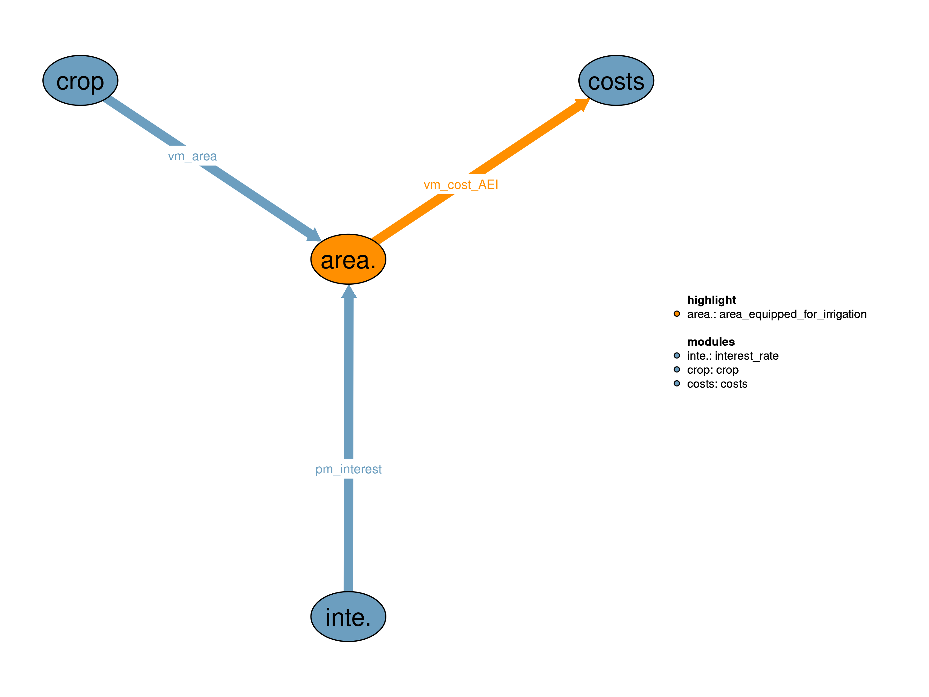
The area equipped for irrigation module constrains irrigated crop production to those areas that are equipped with irrigation infrastructure and simulates the evolution of areas equipped for irrigation. The module receives information about the area actually irrigated from the 30_crop module.
| Description | Unit | A | B | |
|---|---|---|---|---|
| pm_interest (t_all, i) |
Interest rate in each region and timestep | \(\%/yr\) | x | |
| vm_area (j, kcr, w) |
Agricultural production area | \(10^6 ha\) | x | x |
| Description | Unit | |
|---|---|---|
| vm_cost_AEI (i) |
Annuitized irrigation expansion costs | \(10^6 USD_{04MER}/yr\) |
This realization allows the model to endogenously decide on investments to deploy additional irrigation infrastructure, i.e. to increase the area equipped for irrigation (AEI). Initial values for AEI in 1995 are taken from Siebert et al. (2007). Contraction of AEI is not possible. Irrigated crop production can only take place where irrigation infrastructure is present.
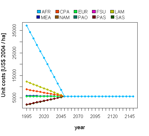
Unit costs per hectare for AEI expansion are derived from a World Bank study (Jones (1995)) and adjusted for the regions used in MAgPIE. The region mapping is as follows:
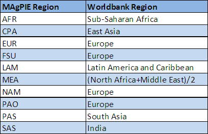
The regional unit costs converge linearly towards the European level until 2050.
\[\begin{multline*} \sum_{kcr} vm\_area(j2,kcr,"irrigated") \leq v41\_AEI(j2) \end{multline*}\]
Investment costs in the current time step for each region are calculated by multiplying the AEI expansion in each cluster of the region by the regional unit cost per hectare and a depreciation rate. MAgPIE has a common planning horizon to which all one time investments are distributed using an annuity approach.
\[\begin{multline*} vm\_cost\_AEI(i2) = \sum_{cell(i2,j2)}\left(v41\_AEI(j2)-pc41\_AEI\_start(j2)\right) \cdot pc41\_unitcost\_AEI(i2) \cdot \left(\left(1-s41\_AEI\_depreciation\right) \cdot \sum_{ct}\left(\frac{pm\_interest(ct,i2)}{\left(1+pm\_interest(ct,i2)\right)}\right) + s41\_AEI\_depreciation\right) \end{multline*}\]
Updating existing capital stocks to account for depreciation
Limitations This realization increases model complexity.
In this realization, area equipped for irrigation is fixed to input data (around the year 2000) for all time steps. The source of the input data is Siebert et al. (2007).
\[\begin{multline*} \sum_{kcr} vm\_area(j2,kcr,"irrigated") \leq v41\_AEI(j2) \end{multline*}\]
This realization assures that irrigated crop production can only take place where irrigation infrastructure is present, i.e. the sum of irrigated cropland vm_area(j,kcr,"irrigated") over all crops in each grid cell has to be less than or equal to the area in this grid cell that is equipped with irrigation infrastructure (v41_AEI(j)).
Limitations No irrigation is possible on areas that have not been equipped for irrigation in the past.
| Description | Unit | A | B | |
|---|---|---|---|---|
| f41_c_irrig (t_all, i) |
Irrigation investment costs | \(USD_{04MER}/ha\) | x | |
| f41_irrig (j) |
Available area equipped for irrigation according to Siebert [AVL] | \(10^6 ha\) | x | x |
| f41_irrig_luh (t_ini41, j) |
Available area equipped for irrigation according to LUH [AVL] | \(10^6 ha\) | x | x |
| p41_AEI_start (t, j) |
Area equipped for irrigation at the beginning of each time step | \(10^6 ha\) | x | |
| pc41_AEI_start (j) |
Area equipped for irrigation at the beginning of current time step | \(10^6 ha\) | x | |
| pc41_unitcost_AEI (i) |
Unit cost of AEI expansion | \(USD_{04MER}/ha\) | x | |
| q41_area_irrig (j) |
Irrigation area constraint | \(10^6 ha\) | x | x |
| q41_cost_AEI (i) |
Calculation of costs of irrigation area expansion | \(10^6 USD_{04MER}\) | x | |
| s41_AEI_depreciation | Depreciation rate in capital value of irrigation infrastructure | x | ||
| v41_AEI (j) |
Area equipped for irrigation in each grid cell | \(10^6 ha\) | x | x |
| description | |
|---|---|
| cell(i, j) | number of LPJ cells per region i |
| ct(t) | Current time period |
| i | all economic regions |
| i2(i) | World regions (dynamic set) |
| j | number of LPJ cells |
| j2(j) | Spatial Clusters (dynamic set) |
| kcr(kve) | Cropping activities |
| t_all(t_ext) | 5-year time periods |
| t_ini41 | Time periods with area equipped for irrigation initialization data |
| t(t_all) | Simulated time periods |
| type | GAMS variable attribute used for the output |
| w | Water supply type |
Anne Biewald, Markus Bonsch, Christoph Schmitz
11_costs, 12_interest_rate, 30_crop, 41_area_equipped_for_irrigation
Jones, William I. 1995. “World Bank and Irrigation.” Washington, D.C.: World Bank.
Siebert, Stefan, Petra Döll, Sebastian Feick, Jippe Hoogeveen, and Karen Frenken. 2007. “Global Map of Irrigation Areas Version 4.0.1.” Johann Wolfgang Goethe University, Frankfurt Am Main, Germany / Food and Agriculture Organization of the United Nations, Rome, Italy. http://www.fao.org/nr/water/aquastat/irrigationmap/index10.stm.