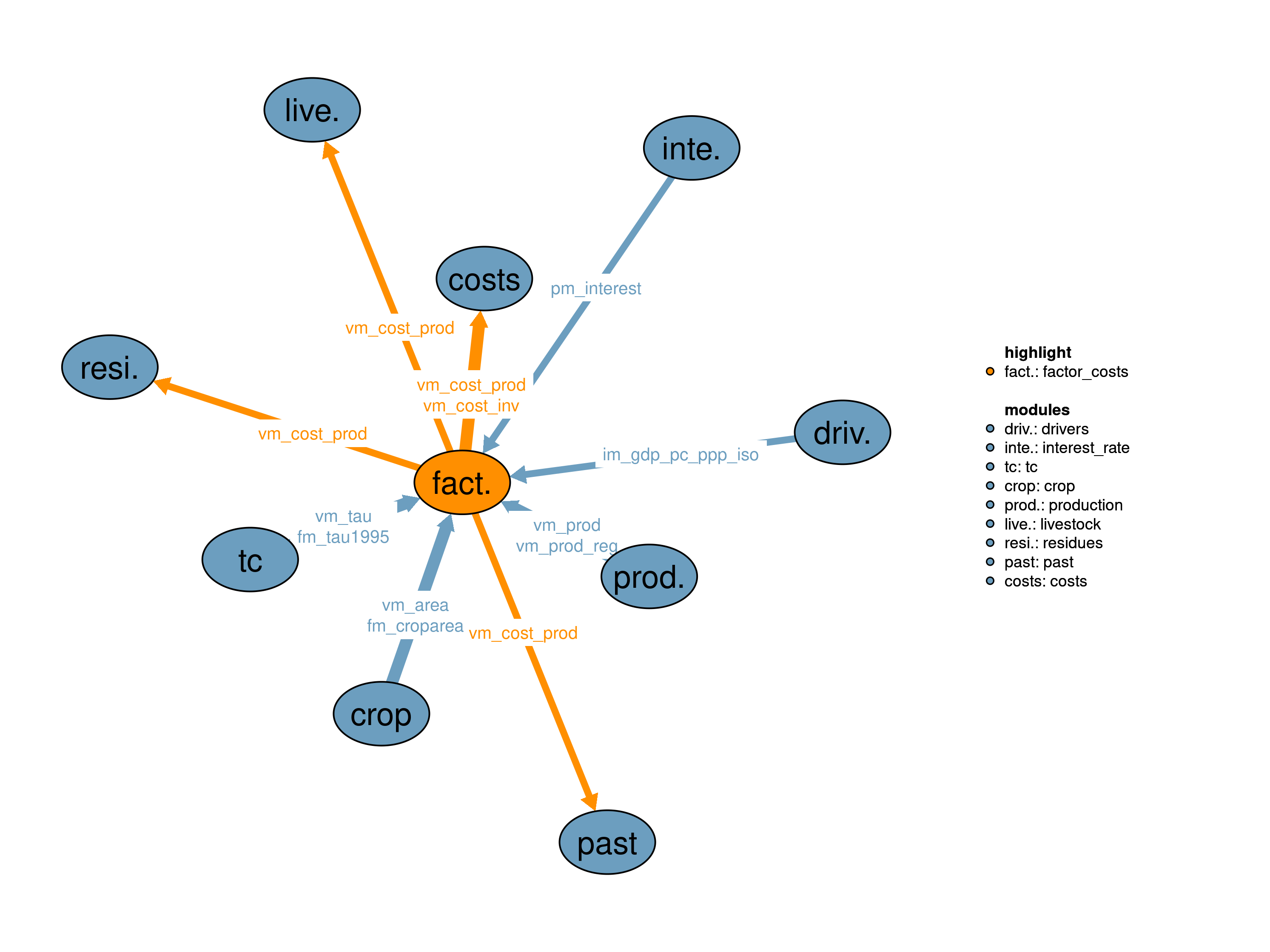
This module is used to calculate factor costs of production in crop activities. The costs of factors of production included in this module are specifically of labor, capital, and energy and related costs. The costs are crop-specific, and pass to the the cost function in 11_costs. Thus, factor costs will contribute to and influence the choice of production pattern in the model.
| Description | Unit | A | B | C | |
|---|---|---|---|---|---|
| fm_croparea (t_all, j, w, kcr) |
Different croparea type areas | \(10^6 ha\) | x | ||
| fm_tau1995 (h) |
Agricultural land use intensity tau in 1995 | \(1\) | x | x | |
| im_gdp_pc_ppp_iso (t_all, iso) |
Per capita income in purchasing power parity | \(USD_{05PPP}/cap/yr\) | x | ||
| pm_interest (t_all, i) |
Interest rate in each region and timestep | \(\%/yr\) | x | ||
| vm_area (j, kcr, w) |
Agricultural production area | \(10^6 ha\) | x | ||
| vm_prod (j, k) |
Production in each cell | \(10^6 tDM/yr\) | x | ||
| vm_prod_reg (i, kall) |
Regional aggregated production | \(10^6 tDM/yr\) | x | x | |
| vm_tau (h) |
Agricultural land use intensity tau | \(1\) | x |
| Description | Unit | |
|---|---|---|
| vm_cost_inv (i) |
Capital investment costs | \(10^6 USD_{05MER} /yr\) |
| vm_cost_prod (i, kall) |
Factor costs | \(10^6 USD_{05MER}/yr\) |
This realization relates factor costs to volume of production of a given crop. The latter 17_production depends on area harvested from 30_crop and yields from 14_yields. In other words, in this implementation, factor costs entirely depend on the volume of production. As such, there are no incentives to allocate and concentrate production into more productive cells.
\[\begin{multline*} vm\_cost\_prod(i2,kcr) = vm\_prod\_reg(i2,kcr) \cdot f38\_fac\_req\_per\_ton(kcr) \end{multline*}\]
The factor requirement costs vm_cost_prod are calculated as product of production quantity vm_prod_reg and crop-specific world average factor costs of production per volume f38_fac_req_per_ton. The volume depending factor costs, which remains fixed overtime, are obtained from value-added costs which correspond to the factor of production included in this module from GTAP7 (Narayanan and Walmsley (2008)). It worth to mention again that the factor costs in this module do not include land rents (as MAgPIE calculates land rents endogenously), chemical fertilizer costs (as they are calculated in 50_nr_soil_budget module), and costs of agricultural intermediate inputs such as seeds (to avoid double counting in the model).
Limitations This realization assumes that factor costs, within a region, purely depend on the production and are independent of the area under cultivation. By implication, cases in which the harvested area could significantly influence factors costs are hardly accounted in this realization.
This ‘mixed’ realization specifies factors costs to depend on area harvested and agricultural land use intensity and corresponding average production volumes. Consequently, factor costs in this realization react on both: area under production and average productivity of a region as captured by the \(\tau\) factor. A detailed description of the approach can be found in Dietrich et al. (2014) with background information about the used intensity measure in Dietrich et al. (2012).
\[\begin{multline*} vm\_cost\_prod(i2,kcr) = \sum_{cell(i2,j2), w}\left( vm\_area(j2,kcr,w) \cdot f38\_region\_yield(i2,kcr) \cdot \sum_{supreg(h2,i2)}\left(\frac{ vm\_tau(h2)}{fm\_tau1995(h2)}\right) \cdot f38\_fac\_req(kcr,w)\right) \end{multline*}\]
The equation above shows that factor requirement costs vm_cost_prod mainly depend on area harvested vm_area and average regional land-use intensity levels vm_tau. Multiplying the land-use intensity increase increases since 1995 with average regional yields f38_region_yield gives the average regional yield. Multiplied with the area under production it gives the production of this location assuming an average yield. Multiplied with estimated factor requirement costs per volume f38_fac_req returns the total factor costs.
The crop-and-water specific factor costs per volume of crop production f38_fac_req are obtained from Narayanan and Walmsley (2008). Splitting factors costs into costs under irrigation and under rainfed production was performed based on the methodology described in Calzadilla, Rehdanz, and Tol (2011).
In this realization, regardless of the cellular productivity, the factor costs per area are identical for all cells within a region. This implicitly gives an incentive to allocate and concentrate production to highly productive cells.
Limitations This realization assumes that factor costs only depend on area and average productivity of a region. Productivity differences within a region are ignored. Therefore, cases in which the cellular productivity levels affect factors costs are only partially accounted for.
The main goal of this realization is to improve crop patterns at different spatial scales. Specifically, the goal is reached by reducing capital relocation flexibility between crop types. In the “sticky” realization, the factor costs are separated into variable and capital investment costs. Then, capital is furtherly divided into immobile and mobile, where mobility is defined between crops. In this way, changes in cropland are favored in locations with existing capital stocks.
Depreciation rate assuming roughly 20 years linear depreciation for invesment goods Share of immobile capital.
Variable costs (without capital): The factor costs are calculated based on the requirements of the regional aggregated production without
\[\begin{multline*} vm\_cost\_prod(i2,kcr) = vm\_prod\_reg(i2,kcr) \cdot \sum_{ct}p38\_variable\_costs(ct,i2,kcr) \end{multline*}\]
Investment costs: Investment are the summation of investment in mobile and immobile capital. The costs are annuitized, and corrected to make sure that the annual depreciation of the current time-step is accounted for.
\[\begin{multline*} vm\_cost\_inv(i2) = \left(\sum_{cell(i2,j2),kcr}v38\_investment\_immobile(j2,kcr) +\sum_{cell(i2,j2)}v38\_investment\_mobile(j2)\right) \cdot \left(\left(1-s38\_depreciation\_rate\right) \cdot \sum_{ct}\left(\frac{pm\_interest(ct,i2)}{\left(1+pm\_interest(ct,i2)\right)}\right) + s38\_depreciation\_rate\right) \end{multline*}\]
Each cropping activity requires a certain capital stock that depends on the production. The following equations make sure that new land expansion is equipped with capital stock, and that depreciation of pre-existing capital is replaced. Since the mobility of capital is defined over crop-type, immobile capital is set over specific crop types and locations.
\[\begin{multline*} v38\_investment\_immobile(j2,kcr) \geq vm\_prod(j2,kcr) \cdot \sum_{cell(i2,j2)}\left(\sum_{ct}p38\_capital\_need(ct,i2,kcr,"immobile")\right)- \sum_{ct}p38\_capital\_immobile(ct,j2,kcr) \end{multline*}\]
On the other hand, the mobile capital is needed by all crop activities in each location, so it is defined over each j2 cell.
\[\begin{multline*} v38\_investment\_mobile(j2) \geq \sum_{cell(i2,j2),kcr}\left(vm\_prod(j2,kcr) \cdot \sum_{ct}p38\_capital\_need(ct,i2,kcr,"mobile")\right)- \sum_{ct}p38\_capital\_mobile(ct,j2) \end{multline*}\]
Estimate capital stock based on capital remuneration Update of existing stocks
Capital update from the last investment
Limitations This realization assumes that factor costs, within a region, purely depend on the production and are independent of the area under cultivation. By implication, cases in which the harvested area could significantly influence factors costs are hardly accounted in this realization.
| Description | Unit | A | B | C | |
|---|---|---|---|---|---|
| f38_fac_req (kcr, w) |
Factor requirement costs | \(USD_{05MER}/tDM\) | x | x | |
| f38_fac_req_per_ton (kcr) |
Factor requirement costs | \(USD_{05MER}/tDM\) | x | ||
| f38_historical_share (t_all, i) |
Historical capital share | x | |||
| f38_reg_parameters (reg) |
Parameters for dynamic regression | x | |||
| f38_region_yield (i, kcr) |
Regional crop yields | \(tDM/ha\) | x | x | |
| p38_capital_cost_share (t, i) |
Capital share for dynamic calculation | \(1\) | x | ||
| p38_capital_immobile (t, j, kcr) |
Preexisting immobile capital stocks before investment | \(10^6 USD05ppp\) | x | ||
| p38_capital_mobile (t, j) |
Preexisting mobile capital stocks before investment | \(10^6 USD05ppp\) | x | ||
| p38_capital_need (t, i, kcr, mobil38) |
Capital requirements for farming with tau equal 1 | \(10^6 USD05ppp\) | x | ||
| p38_croparea_start (j, kcr) |
Agricultural land initialization area | \(10^6 ha\) | x | ||
| p38_share_calibration (i) |
Summation factor used to calibrate calculated capital shares with historical values | \(1\) | x | ||
| p38_variable_costs (t, i, kcr) |
Variable input costs | \(10^6 USD05ppp/input unit\) | x | ||
| q38_cost_prod_crop (i, kcr) |
Regional factor input costs for plant production | \(10^6 USD_{05MER}/yr\) | x | x | x |
| q38_cost_prod_inv (i) |
Regional investment costs in capital | \(10^6 USD05ppp\) | x | ||
| q38_investment_immobile (j, kcr) |
Cellular immobile investments into farm capital | \(10^6 USD05ppp\) | x | ||
| q38_investment_mobile (j) |
Cellular mobile investments into farm capital | \(10^6 USD05ppp\) | x | ||
| s38_depreciation_rate | depreciation rate | \(share of costs\) | x | ||
| s38_immobile | immobile capital | \(share\) | x | ||
| v38_investment_immobile (j, kcr) |
Investment costs in immobile farm capital | \(10^6 USD05ppp/yr\) | x | ||
| v38_investment_mobile (j) |
Investment costs in mobile farm capital | \(10^6 USD05ppp/yr\) | x |
| description | |
|---|---|
| cell(i, j) | number of LPJ cells per region i |
| ct(t) | Current time period |
| h | all superregional economic regions |
| h2(h) | Superregional (dynamic set) |
| i | all economic regions |
| i_to_iso(i, iso) | mapping regions to iso countries |
| i2(i) | World regions (dynamic set) |
| iso | list of iso countries |
| j | number of LPJ cells |
| j2(j) | Spatial Clusters (dynamic set) |
| k(kall) | Primary products |
| kall | All products in the sectoral version |
| kcr(kve) | Cropping activities |
| land | Land pools |
| mobil38 | types of capital |
| reg | regression parameters for dynamic sticky |
| supreg(h, i) | mapping of superregions to its regions |
| t_all(t_ext) | 5-year time periods |
| t(t_all) | Simulated time periods |
| type | GAMS variable attribute used for the output |
| w | Water supply type |
Jan Philipp Dietrich, Benjamin Bodirsky, Kristine Karstens, Edna J. Molina Bacca
09_drivers, 12_interest_rate, 13_tc, 17_production, 18_residues, 30_crop, 31_past, 38_factor_costs, 70_livestock
Calzadilla, Alvaro, Katrin Rehdanz, and Richard S. J. Tol. 2011. “The Gtap-W Model: Accounting for Water Use in Agriculture.” Kiel Working Paper 1745. Kiel: Kiel Institute for the World Economy (IfW). http://hdl.handle.net/10419/54939.
Dietrich, Jan Philipp, Christoph Schmitz, Hermann Lotze-Campen, Alexander Popp, and Christoph Müller. 2014. “Forecasting Technological Change in Agriculture—an Endogenous Implementation in a Global Land Use Model.” Technological Forecasting and Social Change 81: 236–49. https://doi.org/10.1016/j.techfore.2013.02.003.
Dietrich, Jan Philipp, Christoph Schmitz, Christoph Müller, Marianela Fader, Hermann Lotze-Campen, and Alexander Popp. 2012. “Measuring Agricultural Land-Use Intensity – A Global Analysis Using a Model-Assisted Approach.” Ecological Modelling 232 (May): 109–18. https://doi.org/10.1016/j.ecolmodel.2012.03.002.
Narayanan, G. Badri, and Eds. Walmsley Terrie L. 2008. Global Trade, Assistance, and Production: The Gtap 7 Data Base. Center for Global Trade Analysis, Purdue University. http://www.gtap.agecon.purdue.edu/databases/v7/v7_doco.asp.