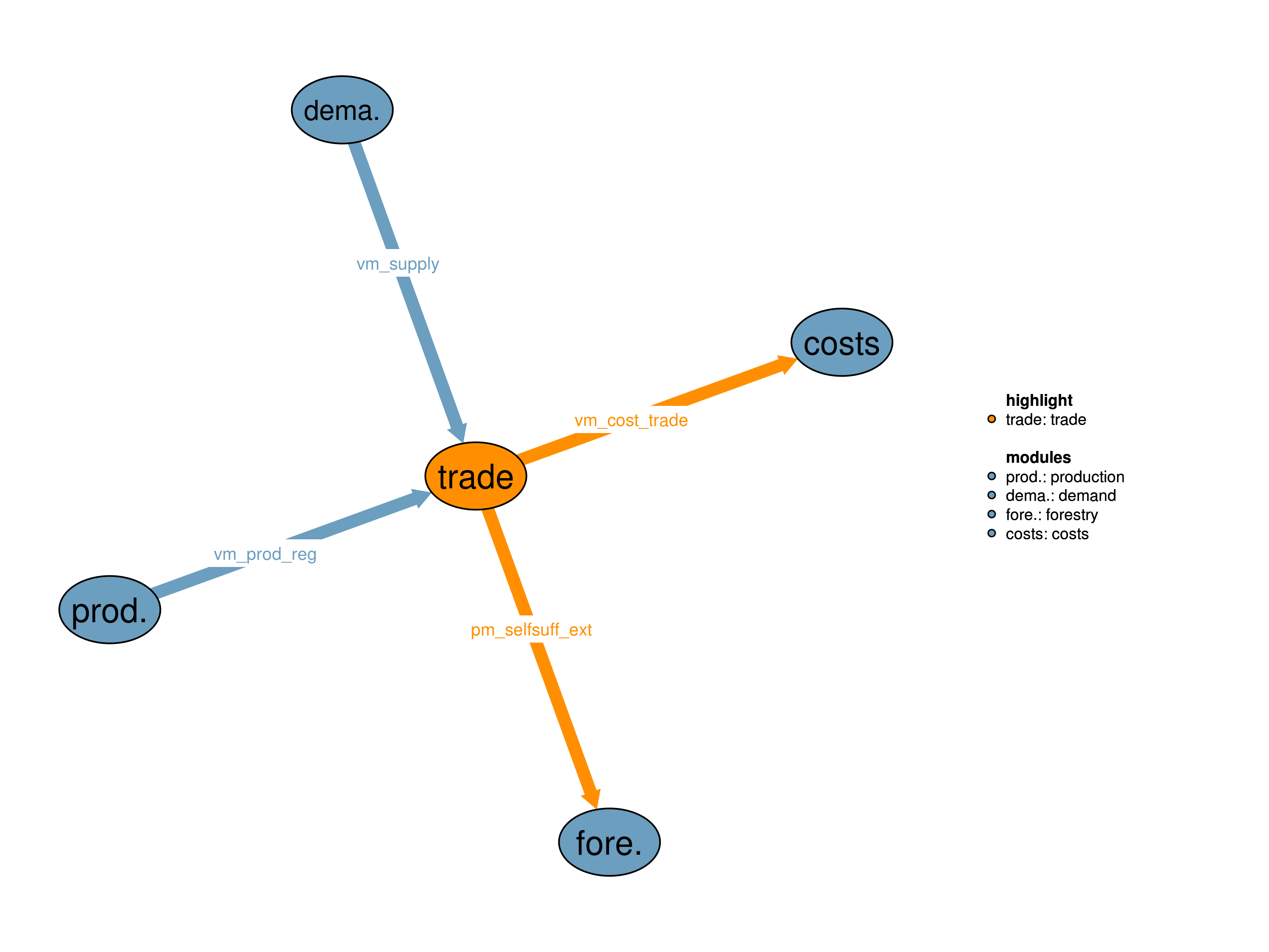
This module represents agricutlural trade among world regions. It ensures that the regional demand is met by domestic production and imports from other regions. The global trade balance dictates that global production must be larger than or equal to global demand. For non-traded goods, the regional production must be larger than or equal to regional demand.

| Description | Unit | A | B | C | D | |
|---|---|---|---|---|---|---|
| vm_prod_reg (i, kall) |
Regional aggregated production | \(10^6 tDM/yr\) | x | x | x | x |
| vm_supply (i, kall) |
Regional demand | \(10^6 tDM/yr\) | x | x | x | x |
| Description | Unit | |
|---|---|---|
| pm_selfsuff_ext (t_ext, h, kforestry) |
Self sufficiency for timber products in extended time frame | \(1\) |
| vm_cost_trade (i) |
Regional trade costs | \(10^6 USD_{05MER}/yr\) |
In this realization, agricultural trade is fully prescribed exogenously. This also means that there is no interaction between regions as amounts of exports and imports are fix.
\[\begin{multline*} \sum_{supreg(h2,i2)}vm\_prod\_reg(i2,kall) \geq \sum_{supreg(h2,i2)} vm\_supply(i2,kall) + \sum_{ct}f21\_trade\_balance(ct,h2,kall) - v21\_manna\_from\_heaven(h2,kall) \end{multline*}\]
The regional production must be bigger than the regional demand plus exports from that region (or minus imports in case of a negative trade balance). As the trade balance in this realization is exogenously defined there is the imminent risk of infeasibilities. To get results even in case of infeasble trade balance conditions v21_manna_from_heaven is introduced. It is an unlimited, but heavily expensive resource which can be used as last resort, if in any other case the model would become infeasible.
\[\begin{multline*} \sum_{supreg(h2,i2)}vm\_cost\_trade(i2) = 10^{6 } \cdot \sum_{kall}v21\_manna\_from\_heaven(h2,kall) \end{multline*}\]
After each run trade costs vm_cost_trade as well as v21_manna_from_heaven should be checked for non-zero values as these will indicate inconsistencies between model simulation and exogenously provided trade balances.
Limitations regions are completely separated and do not interact with each other
In this realization, agricultural trade is fully liberalized in all timesteps.
For traded goods the only active constraint is that the global supply is larger or equal to demand. This means that production can be freely allocated globally based on comparative advantages.
\[\begin{multline*} \sum_{i2 }vm\_prod\_reg(i2,k\_trade) \geq \sum_{i2} vm\_supply(i2,k\_trade) \end{multline*}\]
For non-tradable commodites, the regional supply should be larger or equal to the regional demand.
\[\begin{multline*} \sum_{supreg(h2,i2)}vm\_prod\_reg(i2,k\_notrade) \geq \sum_{supreg(h2,i2)} vm\_supply(i2,k\_notrade) \end{multline*}\]
Limitations This realization does not account for current trends in agricultural trade.
In this realization, there is no agricultural trade, i.e. regions are fully self-sufficient and dependent on domestic production.
For all commodites, the regional supply should be larger or equal to the regional demand.
\[\begin{multline*} \sum_{supreg(h2,i2)}vm\_prod\_reg(i2,kall) \geq \sum_{supreg(h2,i2)} vm\_supply(i2,kall) \end{multline*}\]
Limitations This realization does not account for current trends in agricultural trade.
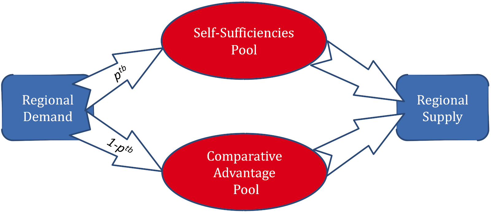
Within this realization, there are two ways for a region to fulfill its demand for agricultural products: a self-sufficiency pool based on historical region specific trade patterns, and a comparative advantage pool based on most cost-efficient production. In the self-sufficiency pool, regional self-sufficiency ratios f21_self_suff_seedred_1995(i,k) defines how much of the demand of each region i for each traded goods k_trade has to be met by domestic production. Self sufficiency ratios smaller than one indicate that the region imports from the world market, while self-sufficiencies greater than one indicate that the region produces for export. Trade costs, inlucding trade margins and tariffs, are considered.

In the comparative advantage pool, the only active constraint is that the global supply is larger or equal to demand. This means that production can be freely allocated globally based on comparative advantages.
\[\begin{multline*} \sum_{i2 }vm\_prod\_reg(i2,k\_trade) \geq \sum_{i2} vm\_supply(i2,k\_trade) + \sum_{ct}f21\_trade\_balanceflow(ct,k\_trade) \end{multline*}\]
For non-tradable commodites, the regional supply should be larger or equal to the regional demand.
\[\begin{multline*} \sum_{supreg(h2,i2)}vm\_prod\_reg(i2,k\_notrade) \geq \sum_{supreg(h2,i2)} vm\_supply(i2,k\_notrade) \end{multline*}\]
The following equation indicates the regional trade constraint for the self-sufficiency pool. The share of regional demand that has to be fulfilled through the self-sufficiency pool is determined by a trade balance reduction factor for each commodity i21_trade_bal_reduction(ct,k_trade) according to the following equations (Schmitz et al. 2012). If the trade balance reduction equals 1 (f21_self_suff(ct,i2,k_trade) = 1), all demand enters the self-sufficiency pool. If it equals 0, all demand enters the comparative advantage pool. Lower bound for production.
\[\begin{multline*} \sum_{supreg(h2,i2)}vm\_prod\_reg(i2,k\_trade) \geq \left(\sum_{supreg(h2,i2)}vm\_supply(i2,k\_trade) + v21\_excess\_prod(h2,k\_trade)\right) \cdot \sum_{ct}i21\_trade\_bal\_reduction(ct,k\_trade) \$\left(\sum_{ct}\left(f21\_self\_suff(ct,h2,k\_trade) \geq 1\right)\right) + \sum_{supreg(h2,i2)}vm\_supply(i2,k\_trade) \cdot \sum_{ct}f21\_self\_suff(ct,h2,k\_trade) \cdot \sum_{ct}i21\_trade\_bal\_reduction(ct,k\_trade) \$\left(\sum_{ct}\left(f21\_self\_suff(ct,h2,k\_trade) < 1\right)\right) \end{multline*}\]
Upper bound for production.
\[\begin{multline*} \sum_{supreg(h2,i2)}vm\_prod\_reg(i2,k\_trade) \leq \left(\frac{\left(\sum_{supreg(h2,i2)}vm\_supply(i2,k\_trade) + v21\_excess\_prod(h2,k\_trade)\right)}{\sum_{ct}i21\_trade\_bal\_reduction(ct,k\_trade)}\right) \$\left(\sum_{ct}\left(f21\_self\_suff(ct,h2,k\_trade) \geq 1\right)\right) + \left(\sum_{supreg(h2,i2)}vm\_supply(i2,k\_trade) \cdot \frac{\sum_{ct}f21\_self\_suff(ct,h2,k\_trade)}{\sum_{ct}i21\_trade\_bal\_reduction(ct,k\_trade)}\right) \$\left(\sum_{ct}\left(f21\_self\_suff(ct,h2,k\_trade) < 1\right)\right) \end{multline*}\]
The global excess demand of each tradable good v21_excess_demad equals to the sum over all the imports of importing regions.
\[\begin{multline*} v21\_excess\_dem(k\_trade) \geq \sum_{h2}\left( \sum_{supreg(h2,i2)}vm\_supply(i2,k\_trade) \cdot \left(1 - \sum_{ct}f21\_self\_suff(ct,h2,k\_trade)\right) \$\left(\sum_{ct}f21\_self\_suff(ct,h2,k\_trade) < 1\right)\right) + \sum_{ct}f21\_trade\_balanceflow(ct,k\_trade) \end{multline*}\]
Distributing the global excess demand to exporting regions is based on regional export shares (Schmitz et al. 2012). Export shares are derived from FAO data (see Schmitz et al. (2012) for details). They are 0 for importing regions.
\[\begin{multline*} v21\_excess\_prod(h2,k\_trade) = v21\_excess\_dem(k\_trade) \cdot \sum_{ct}f21\_exp\_shr(ct,h2,k\_trade) \end{multline*}\]
\[\begin{multline*} v21\_cost\_trade\_reg(h2,k\_trade) \geq \left(i21\_trade\_margin(h2,k\_trade) + i21\_trade\_tariff(h2,k\_trade)\right) \cdot \sum_{supreg(h2,i2)}\left( vm\_prod\_reg(i2,k\_trade)-vm\_supply(i2,k\_trade)\right) \end{multline*}\]
\[\begin{multline*} \sum_{supreg(h2,i2)}vm\_cost\_trade(i2) = \sum_{k\_trade}v21\_cost\_trade\_reg(h2,k\_trade) \end{multline*}\]
Limitations This realization depends on predetermined self-sufficiency rates and export shares, which leads to a relative fixed trade pattern.
| Description | Unit | A | B | C | D | |
|---|---|---|---|---|---|---|
| f21_exp_shr (t_all, h, kall) |
Superregional and crop-specific export share | \(1\) | x | |||
| f21_self_suff (t_all, h, kall) |
Superregional self-sufficiency rates | \(1\) | x | x | x | x |
| f21_trade_bal_reduction (t_all, trade_groups21, trade_regime21) |
Share of inelastic trade pool | \(1\) | x | |||
| f21_trade_balance (t_all, h, kall) |
trade balance of positive exports and negative imports | \(10^6 tDM/yr\) | x | x | ||
| f21_trade_balanceflow (t_all, kall) |
Domestic balance flows | \(10^6 tDM/yr\) | x | |||
| f21_trade_margin (h, kall) |
Costs of freight and insurance | \(USD_{05MER}/tDM\) | x | |||
| f21_trade_tariff (h, kall) |
Specific duty tariffs | \(USD_{05MER}/tDM\) | x | |||
| i21_trade_bal_reduction (t_all, k_trade) |
Trade balance reduction | \(1\) | x | x | ||
| i21_trade_margin (h, k_trade) |
Trade margins | \(USD_{05MER}/tDM\) | x | x | ||
| i21_trade_tariff (h, k_trade) |
Trade tariffs | \(USD_{05MER}/tDM\) | x | x | ||
| q21_cost_trade (h) |
Superregional trade costs | \(10^6 USD_{05MER}/yr\) | x | x | ||
| q21_cost_trade_reg (h, k_trade) |
Superregional trade costs for each tradable commodity | \(10^6 USD_{05MER}/yr\) | x | |||
| q21_excess_dem (k_trade) |
Global excess demand | \(10^6 tDM/yr\) | x | |||
| q21_excess_supply (h, k_trade) |
Superregional excess production | \(10^6 tDM/yr\) | x | |||
| q21_notrade (h, kall) |
Superregional production constraint of non-tradable commodities | \(10^6 tDM/yr\) | x | x | x | x |
| q21_trade_glo (k_trade) |
Global production constraint | \(10^6 tDM/yr\) | x | x | ||
| q21_trade_reg (h, k_trade) |
Superregional trade balances i.e. minimum self-sufficiency ratio | \(1\) | x | |||
| q21_trade_reg_up (h, k_trade) |
Superregional trade balances i.e. maximum self-sufficiency ratio | \(1\) | x | |||
| s21_trade_bal_damper | Fraction to ease self sufficiency pool trade for roundwood | x | ||||
| s21_trade_tariff | Trade tariff switch (1=on 0=off) | \(1\) | x | |||
| v21_cost_trade_reg (h, k_trade) |
Superregional trade costs for each tradable commodity | \(10^6 USD_{05MER}/yr\) | x | |||
| v21_excess_dem (k_trade) |
Global excess demand | \(10^6 tDM/yr\) | x | |||
| v21_excess_prod (h, k_trade) |
Superregional excess production | \(10^6 tDM/yr\) | x | |||
| v21_manna_from_heaven (h, kall) |
Last resort resource for otherwise infeasible trade balance constraints | \(10^6 tDM/yr\) | x |
| description | |
|---|---|
| ct(t) | Current time period |
| h | all superregional economic regions |
| h2(h) | Superregional (dynamic set) |
| i | all economic regions |
| i2(i) | World regions (dynamic set) |
| k_hardtrade21(k_trade) | Products where trade should be limited |
| k_notrade(kall) | Production activities of non-tradable commodites |
| k_trade(kall) | Production activities of tradable commodities |
| kall | All products in the sectoral version |
| kforestry(k) | forestry products |
| supreg(h, i) | mapping of superregions to its regions |
| t_all(t_ext) | 5-year time periods |
| t_ext | 5-year time periods |
| t(t_all) | Simulated time periods |
| trade_groups21 | Trade groups |
| trade_regime21 | Trade scenarios |
| tstart21(t_all) | Historic time steps |
| type | GAMS variable attribute used for the output |
Xiaoxi Wang, Anne Biewald, Christoph Schmitz, Markus Bonsch
11_costs, 16_demand, 17_production, 32_forestry