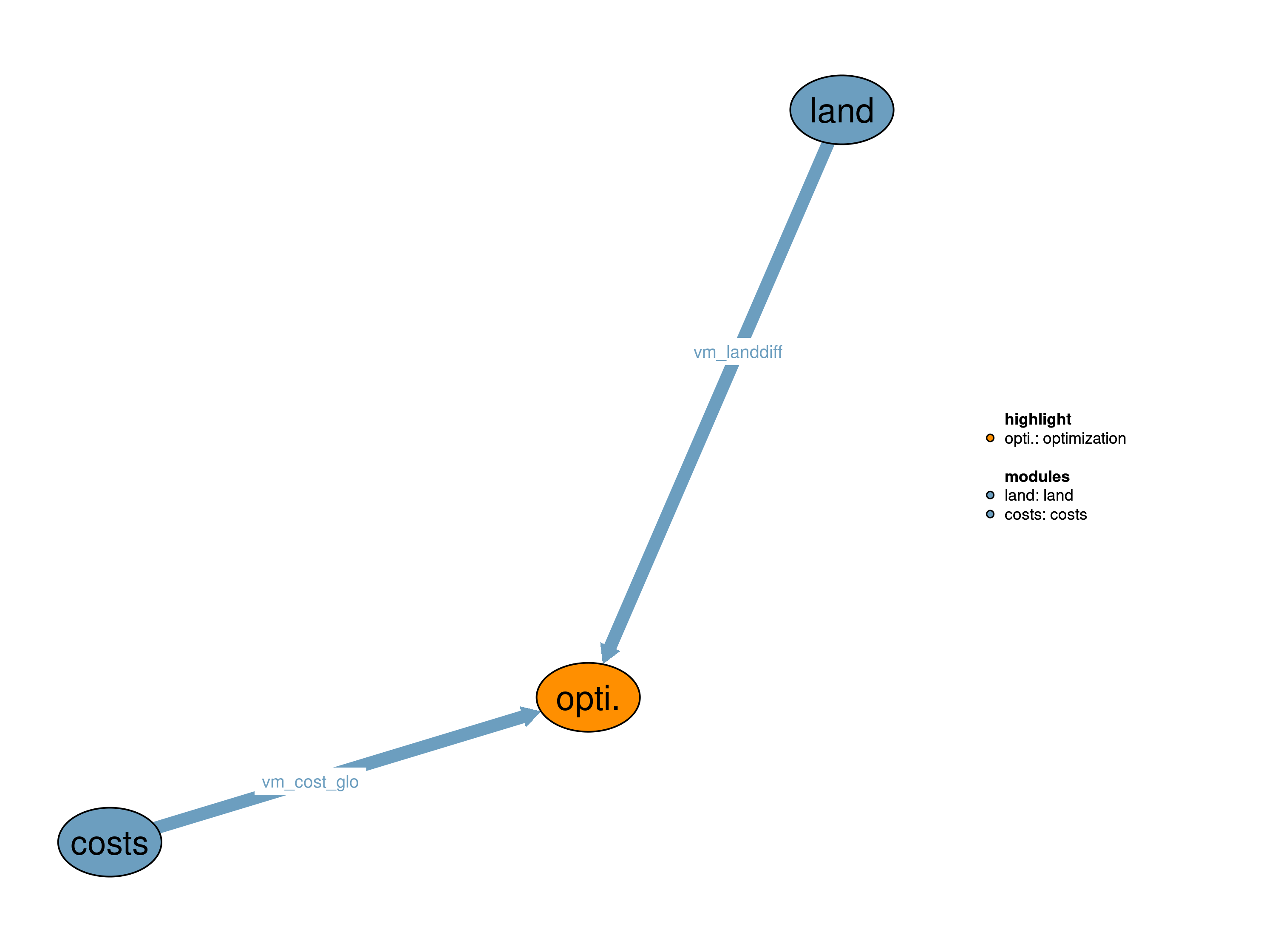
This module takes care of the model optimization of the main model, allowing for switching between optimization procedures. It has been introduced to play with different ways to affect the runtime performance of the model via more optimized model solution strategies. The interfaces to the rest of the model are quite limited as it only requires the variables to be optimized vm_cost_glo (total costs) and vm_landdiff (gross land use changes compared to last time step) as direct input. The latter was introduced to select out of a range of cost optimal patterns that one which is closest to the pattern of the previous time step. While CONOPT returns this solution by default, CPLEX does not.
| Description | Unit | A | B | C | |
|---|---|---|---|---|---|
| vm_cost_glo | Total costs of production | \(10^6 USD_{05MER}/yr\) | x | x | x |
| vm_landdiff | Aggregated difference in land between current and previous time step | \(10^6 ha\) | x |
In this realization, instead of directly starting the nonlinear optimization, a linear version of the model is solved beforehand. In order to linearize the model all nonlinear terms are fixed to best guesses for the respective values. The linear solution serves as an improved starting point for the nonlinear optimization.
All nonlinear terms are fixed to best guess values via nl_fix.gms files which must be provided for each nonlinear module realization.
$batinclude "./modules/include.gms" nl_fixAfter all nonlinearities have been fixed the linear model is solved. Via setting magpie.trylinear = 1 the following solve statement starts a linear optimization if no non-linearities remain in the model (Please note that the solve statement still declares a nonlinear / nlp problem even though we expect it to be linear!).
solve magpie USING nlp MINIMIZING vm_cost_glo;A second optimization makes sure that in case of a flat optimum that solution is chosen for which the difference in land changes compared to the previous timestep is minimized. This is achieved by setting the calculated total costs of the previous optimization as upper bound and minimizing the land differences.
    if((magpie.modelstat=1 or magpie.modelstat = 7),
      vm_cost_glo.up = vm_cost_glo.l;
      solve magpie USING nlp MINIMIZING vm_landdiff;
      vm_cost_glo.up = Inf;
    );
After the linear optimization all nonlinear variables are released again.
$batinclude "./modules/include.gms" nl_releaseIn case that no feasible solution for the linear model is found the best guess estimates for the fixations of nonlinear terms are slightly relaxed to increase the likelihood of finding a feasible solution and the linear solve is repeated. Such as the nl_fix.gms and nl_release.gms rules also nl_release.gms must be provided by the corresponding module realizations.
    if((p80_modelstat(t) <> 1),
$batinclude "./modules/include.gms" nl_relax
    );
Finally, the linear solution is used as starting point for the nonlinear optimization of the model in its full complexity.
solve magpie USING nlp MINIMIZING vm_cost_glo;Limitations This realization requires that all module realizations with nonlinear terms provide a
nl_fix.gmsandnl_release.gmswhich fix and release all nonlinear terms in the module. If this is missing and there are still active, nonlinear terms in the linear solve attempt the model run will be cancelled by an error.
In this realization the model is solved directly using nonlinear optimization. If the optimization returns an infeasible solution the solve is repeated, either until a feasible solution is found or the maximum number of iterations as defined in s80_maxiter is reached.
solve magpie USING nlp MINIMIZING vm_cost_glo;Limitations There are no known limitations.
In this realization the model is solved directly using nonlinear optimization. However, the regions are solved in parallel. This allows to use higher spatial resolution, but works only with fixed trade patterns (exo trade realization). To derive these trade patterns a normal run with global optimization is needed. The start script highres.R illustrates how this can be used. If the optimization returns an infeasible solution the solve is repeated, either until a feasible solution is found or the maximum number of iterations as defined in s80_maxiter is reached.
Limitations There are no known limitations.
| Description | Unit | A | B | C | |
|---|---|---|---|---|---|
| p80_counter (i) |
counter | \(1\) | x | ||
| p80_handle (i) |
parallel mode handle parameter | \(1\) | x | ||
| p80_modelstat (t) |
modelstat indicator | \(1\) | x | x | x |
| p80_num_nonopt (t) |
numNOpt indicator | \(1\) | x | x | x |
| s80_add_conopt3 | add conopt3 optimization after conopt4 | \(1\) | x | ||
| s80_add_cplex | add cplex optimization after conopt4 | \(1\) | x | ||
| s80_counter | counter | \(1\) | x | x | |
| s80_maxiter | maximal solve iterations if modelstat is > 2 | \(1\) | x | x | x |
| s80_num_nonopt_allowed | number of allowed non-optimal variables | \(1\) | x | x | x |
| s80_obj_linear | linear objective value | \(10^6 USD_{05MER}/yr\) | x | ||
| s80_optfile | switch to use specfied solver settings | \(1\) | x | x | x |
| description | |
|---|---|
| cell(i, j) | number of LPJ cells per region i |
| i | all economic regions |
| i2(i) | World regions (dynamic set) |
| j | number of LPJ cells |
| j2(j) | Spatial Clusters (dynamic set) |
| t(t_all) | Simulated time periods |
Jan Philipp Dietrich, Todd Munson