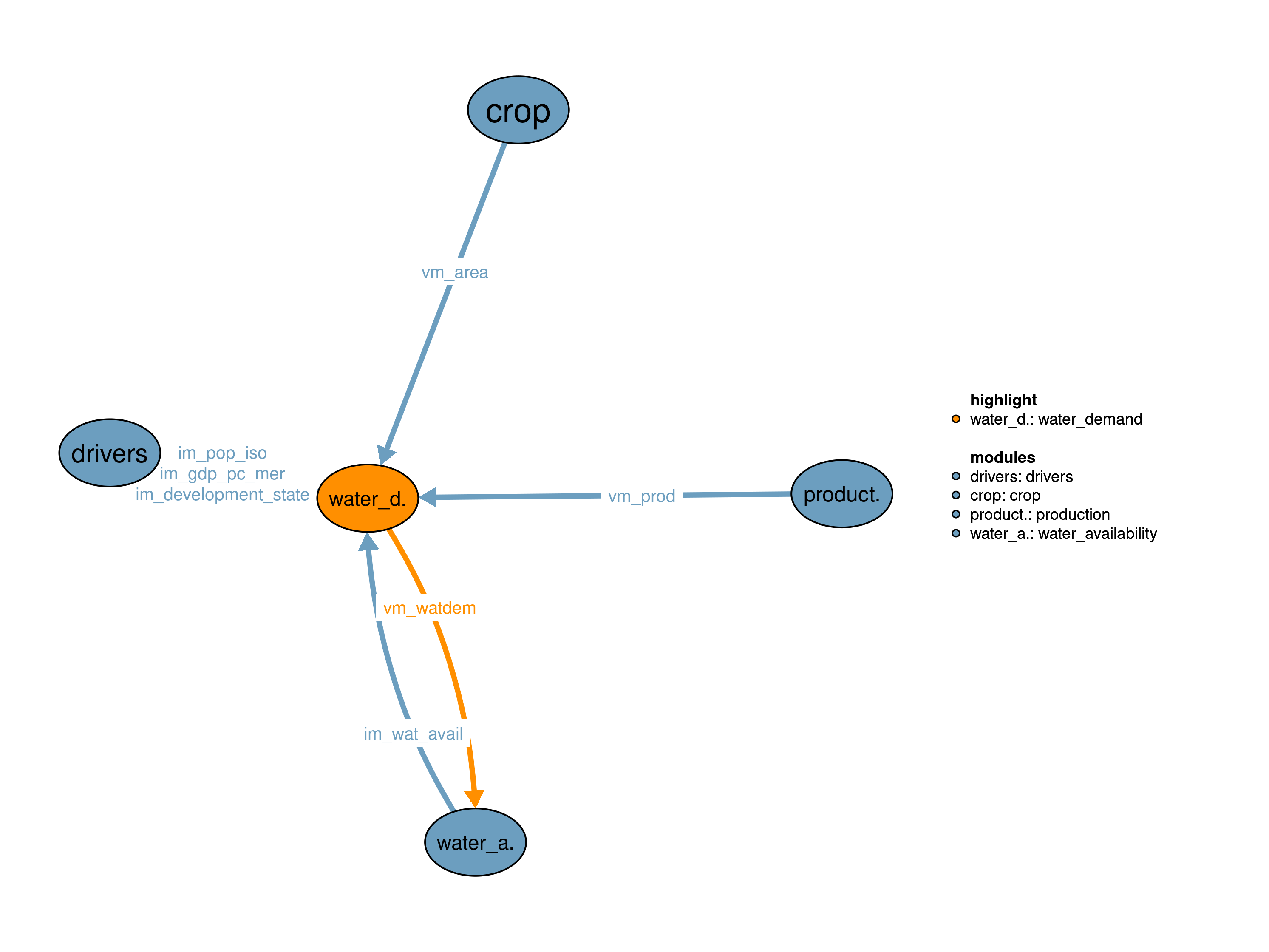
The water demand module determines the water demand in the following sectors: agriculture, industry, electricity, domestic and ecosystem. Different scenarios for different water demand and environmental flow protection are possible. The module receives information from the 17_production, 30_crop, 09_drivers and 43_water_availability modules. It passes information to the module 43_water_availability and 11_costs.
| Description | Unit | A | B | |
|---|---|---|---|---|
| im_development_state (t_all, i) |
Development state according to the World Bank definition where 0=low income country 1=high income country in high income level | \(1\) | x | x |
| im_gdp_pc_mer (t_all, i) |
Per capita income in market exchange rates | \(USD_{05MER}/cap/yr\) | x | x |
| im_pop_iso (t_all, iso) |
Population | \(10^6/yr\) | x | x |
| im_wat_avail (t, wat_src, j) |
Water availability | \(10^6 m^3/yr\) | x | x |
| sm_fix_SSP2 | year until which all parameters are fixed to SSP2 values | \(year\) | x | x |
| vm_area (j, kcr, w) |
Agricultural production area | \(10^6 ha\) | x | x |
| vm_prod (j, k) |
Production in each cell | \(10^6 tDM/yr\) | x | x |
| Description | Unit | |
|---|---|---|
| vm_watdem (wat_dem, j) |
Water demand from different sectors | \(10^6 m^3/yr\) |
This realization models agricultural sector water demand endogenously, while other sectors are kept exogenous; Various settings for environmental water demand described below.
Agricultural water demand:
Water demand for agriculture is endogenously calculated based on irrigated cropland vm_area(j,kcr,"irrigated") and livestock production vm_prod(j2,kli).
Irrigation water demand per area for each crop category and cluster is provided by the LPJmL model. This parameter refers to the water that has to be applied to the field, i.e. it includes losses due to evaporation on the field, but does not include losses during the water transport from source to field. Livestock water demand ic42_wat_req_k(j,kli) is derived from FAO data.
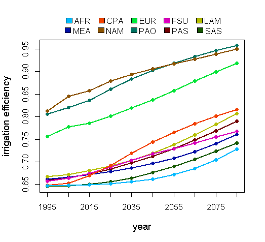
Irrigation efficiency:
Switches for different scenarios for irrigation efficiency can be chosen:
A global static value of irrigation efficiency that is defined as the global weighted average of water losses from source to field (“conveyance efficiency times management factor”) from Rohwer, Gerten, and Lucht (2007). Here, irrigated area from Siebert et al. (2007) has been used as aggregation weight.
A regression of country values of the “conveyance efficiency times management factor” from Rohwer, Gerten, and Lucht (2007) on GDP.
Non agricultural human water demand:
Water demand from all other sectors is treated exogenously. The scalar s42_reserved_fraction determines how much water is reserved for non agricultural purposes. Technically, it is assigned to industrial use, while demand for other non-agricultural sectors is set to 0. The default value is 0.5.
Environmental water demand
Environmental water requirements can be specified separately using the switch s42_env_flow_scenario. The following settings are available:
s42_env_flow_fraction is reserved for environmental purposes and consequently not available for agricultural activities (in addition to s42_reserved_fraction).s42_protected_fraction. In the case of the absence of an environmental flow protection (EFP) policy, a base protection can be specified: s42_env_flow_base_fraction. Its default value is 5 % of available water.Whether a potential EFP policy takes effect is determined by the parameter f42_env_flow_policy.
\[\begin{multline*} vm\_watdem("agriculture",j2) \cdot v42\_irrig\_eff(j2) = \sum_{kcr}\left( vm\_area(j2,kcr,"irrigated") \cdot ic42\_wat\_req\_k(j2,kcr)\right) + \sum_{kli}\left(vm\_prod(j2,kli) \cdot ic42\_wat\_req\_k(j2,kli) \cdot v42\_irrig\_eff(j2)\right) \end{multline*}\]
vm_watdem is composed by irrigation and livestock demand uses. The factor v42_irrig_eff corresponds to the amount of water that is used inefficiently in the irrigation process.
Limitations The module uses the “conveyance efficiency times management factor” for irrigation efficiency. Therefore, the management factor is accounted twice, since it is already considered in LPJmL water quantity used for irrigation (
airrig: annual irrigation). Furthermore, the module realization does not consider annual water balances but only water balances during the growing period of crops. This period differs between cells.
This realization models agricultural sector water demand endogenously, as described in the first realization, Industry, electricity and domestic demand are also modelled endogenously with various scenarios; Various settings (same ias in previous realization) for environmental water demand described below.
Agricultural water demand:
Water demand for agriculture is endogenously calculated based on irrigated cropland vm_area(j,kcr,"irrigated") and livestock production vm_prod(j,kli).
Non agricultural human water demand:
For industry, electricity and domestic demand, three scenarios are available on cluster level from the model by Alcamo et al. (2003):
Due to the fact that MAgPIE only considers available blue water during the growing period of the plants (43_water_availability), the fraction of this demand in the growing period is determined in the preprocessing assuming constant demand over the whole year. The matching of the WATERGAP scenarios to the MAgPIE scenarios can be found in the file scenario_config.csv in the config folder of model.
Environmental water demand:
Environmental water requirements can be specified separately using the switch s42_env_flow_scenario. The following settings are available:
s42_env_flow_fraction is reserved for environmental purposes and consequently not available for agricultural activities (in addition to s42_reserved_fraction).s42_protected_fraction. In the case of the absence of an environmental flow protection policy, a base protection can be specified: s42_env_flow_base_fraction. It defaults to 5 % of available water.\[\begin{multline*} vm\_watdem("agriculture",j2) \cdot v42\_irrig\_eff(j2) = \sum_{kcr}\left( vm\_area(j2,kcr,"irrigated") \cdot ic42\_wat\_req\_k(j2,kcr)\right) + \sum_{kli}\left(vm\_prod(j2,kli) \cdot ic42\_wat\_req\_k(j2,kli) \cdot v42\_irrig\_eff(j2)\right) \end{multline*}\]
vm_watdem is composed by irrigation and livestock demand uses. The factor v42_irrig_eff corresponds to the amount of water that is used inefficiently in the irrigation process.
Limitations The module uses the “conveyance efficiency times management factor” for irrigation efficiency. Therefore, the management factor is accounted twice, since it is already considered in LPJmL water quantity used for irrigation (
airrig: annual irrigation). Furthermore, the module realization does not consider annual water balances but only water balances during the growing period of crops. This period differs between cells.
| Description | Unit | A | B | |
|---|---|---|---|---|
| f42_env_flow_policy (t_all, scen42) |
EFP policies | \(1\) | x | x |
| f42_env_flows (t_all, j) |
Environmental flow requirements from LPJ and Smakhtin algorithm | \(10^6 m^3\) | x | x |
| f42_wat_req_kli (kli) |
Average water requirements of livestock commodities per region per tDM per year | \(m^3\) | x | x |
| f42_wat_req_kve (t_all, j, kve) |
LPJmL annual water demand for irrigation per ha | \(m^3/yr\) | x | x |
| f42_watdem_ineldo (t_all, j, scen_watdem_nonagr, watdem_ineldo) |
Industry electricity and domestic water demand under our socioeconomic scenarios | \(10^6 m^3\) | x | |
| i42_env_flow_policy (t, i) |
Determines whether environmental flow protection is enforced | \(1\) | x | x |
| i42_env_flows (t, j) |
Environmental flow requirements if a protection policy is in place | \(10^6 m^3\) | x | x |
| i42_env_flows_base (t, j) |
Environmental flow requirements if no protection policy is in place | \(10^6 m^3\) | x | x |
| i42_wat_req_k (t, j, k) |
LPJmL annual water demand for irrigation per ha per year (m^3) + Livestock demand per ton | \(m^3\) | x | x |
| ic42_env_flow_policy (i) |
Determines whether environmental flow protection is enforced in the current time step | \(1\) | x | x |
| ic42_wat_req_k (j, k) |
LPJmL annual water demand for irrigation per ha per year (m^3) + Livestock demand per ton | \(m^3\) | x | x |
| p42_country_dummy (iso) |
Dummy parameter indicating whether country is affected by EFP | \(1\) | x | x |
| p42_EFP_region_shr (t_all, i) |
Weighted share of region with regards to EFP | \(1\) | x | x |
| q42_water_demand (wat_dem, j) |
Water consumption in different sectors | \(10^6 m^3/yr\) | x | x |
| s42_env_flow_base_fraction | Fraction of available water that is reserved for the environment where no EFP policy is implemented | \(1\) | x | x |
| s42_env_flow_fraction | Fraction of available water that is reserved for under protection policies | \(1\) | x | x |
| s42_env_flow_scenario | EFP scenario. | \(1\) | x | x |
| s42_irrig_eff_scenario | Scenario for irrigation efficiency | \(1\) | x | x |
| s42_irrigation_efficiency | Value of irrigation efficiency | \(1\) | x | x |
| s42_reserved_fraction | Fraction of available water that is reserved for industry electricity and domestic use | \(1\) | x | |
| s42_watdem_nonagr_scenario | Scenario for non agricultural water demand from WATERGAP | \(1\) | x | |
| v42_irrig_eff (j) |
Irrigation efficiency | \(1\) | x | x |
| description | |
|---|---|
| cell(i, j) | number of LPJ cells per region i |
| dev | Economic development status |
| EFP_countries(iso) | countries to be affected by EFP |
| i | all economic regions |
| i_to_iso(i, iso) | mapping regions to iso countries |
| iso | list of iso countries |
| j | number of LPJ cells |
| j2(j) | Spatial Clusters (dynamic set) |
| k(kall) | Primary products |
| kcr(kve) | Cropping activities |
| kli(kap) | Livestock products |
| kve(k) | Land-use activities |
| scen_watdem_nonagr | Scenarios for non agricultural water demand |
| scen42 | Environmental Flow Policy (EFP) |
| scen42_to_dev(scen42, dev) | Mapping between EFP and economic development status |
| t_all | 5-year time periods |
| t(t_all) | Simulated time periods |
| type | GAMS variable attribute used for the output |
| w | Water supply type |
| wat_dem | Water demand sectors |
| wat_src | Type of water source |
| watdem_exo(wat_dem) | Exogenous water demands |
| watdem_ineldo(wat_dem) | Exogenous water demand subset covering humanly induced demands |
Anne Biewald, Markus Bonsch
09_drivers, 17_production, 30_crop, 42_water_demand, 43_water_availability
Alcamo, J., P. DÖLL, T. Henrichs, and et al. 2003. “Development and Testing of the Watergap 2 Global Model of Water Use and Availability.” Hydrological Sciences Journal 48 (3): 317–37.
Rohwer, Janine, Dieter Gerten, and Wolfgang Lucht. 2007. “DEVELOPMENT of Functional Irrigation Types for Improved Global Crop Modelling.” Potsdam: PIK.
Siebert, Stefan, Petra Döll, Sebastian Feick, Jippe Hoogeveen, and Karen Frenken. 2007. “Global Map of Irrigation Areas Version 4.0.1.” Johann Wolfgang Goethe University, Frankfurt Am Main, Germany / Food and Agriculture Organization of the United Nations, Rome, Italy. http://www.fao.org/nr/water/aquastat/irrigationmap/index10.stm.
Smakhtin, V., C. Revenga, P. Döll, and et al. 2004. Taking into Account Environmental Water Requirements in Global-Scale Water Resources Assessments.