
The yields module simulates the temporal development of crop yields and pasture productivity. Spatially explicit information on pasture productivity and crop yields under both rainfed and irrigated conditions is provided by the global gridded crop model LPJmL (Lund-Potsdam-Jena with managed Land) (Bondeau et al. 2007). In the initial year of the simulation period, crop yields and pasture productivity are calibrated at the regional level to meet the observed cropland and pasture area as reported by FAO (FAOSTAT 2016). For the simulation of the temporal development of agricultural yields, the module receives information about the agricultural land use intensity represented by the \(\tau\) factor coming from the module 13_tc. Irrigated yields can optionally be calibrated to meet irrigated-rainfed country-level yield ratios as reported by Aquastat (FAO 2016).
The module returns yields for all crops and for pasture, which is then used by the modules [30_crop] and 31_past.
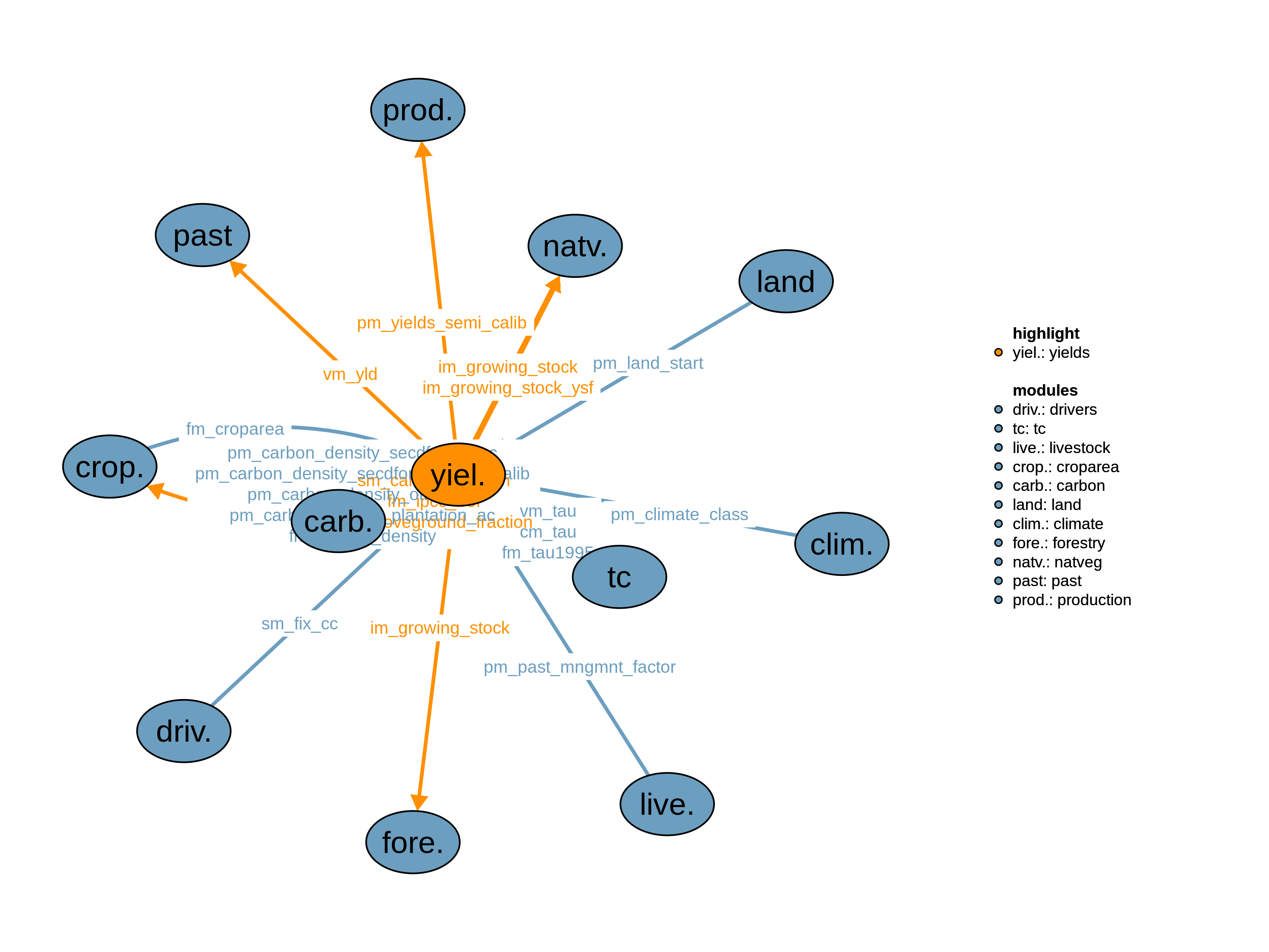
| Description | Unit | A | B | |
|---|---|---|---|---|
| fm_carbon_density (t_all, j, land, c_pools) |
LPJmL carbon density for land and carbon pools | \(tC/ha\) | x | x |
| fm_croparea (t_all, j, w, kcr) |
Different croparea type areas | \(10^6 ha\) | x | x |
| fm_tau1995 (h) |
Agricultural land use intensity tau in 1995 | \(1\) | x | x |
| pcm_tau (j, tautype) |
Tau factor of the previous time step | \(1\) | x | x |
| pm_carbon_density_other_ac (t_all, j, ac, ag_pools) |
Vegetation other land carbon density for age classes and carbon pools | \(tC/ha\) | x | x |
| pm_carbon_density_plantation_ac (t_all, j, ac, ag_pools) |
Vegetation plantation carbon density for age classes and carbon pools | \(tC/ha\) | x | x |
| pm_carbon_density_secdforest_ac (t_all, j, ac, ag_pools) |
Vegetation secondary forest carbon density for age classes and carbon pools | \(tC/ha\) | x | x |
| pm_carbon_density_secdforest_ac_uncalib (t_all, j, ac, ag_pools) |
Vegetation secondary forest carbon density uncalibrated | \(tC/ha\) | x | x |
| pm_climate_class (j, clcl) |
Koeppen-Geiger climate classification on the simulation cluster level | \(1\) | x | x |
| pm_land_start (j, land) |
Land initialization area | \(10^6 ha\) | x | x |
| pm_past_mngmnt_factor (t, i) |
Regional pasture management intensification factor | \(1\) | x | x |
| sm_fix_cc | year until which all parameters affected by cc are fixed to historical values | \(year\) | x | x |
| vm_tau (j, tautype) |
Overall agricultural land use intensity tau at cluster level | \(1\) | x | x |
| Description | Unit | |
|---|---|---|
| fm_aboveground_fraction (land_timber) |
Aboveground fraction of total biomass | \(1\) |
| fm_ipcc_bef (clcl) |
IPCC biomass expansion factor BEF | \(1\) |
| im_growing_stock (t, j, ac, land_timber) |
Harvestable stem biomass per ha by age class | \(tDM/ha\) |
| im_growing_stock_ysf (t, j, ac) |
Harvestable stem biomass per ha by age class for young secondary forest on other land | \(tDM/ha\) |
| pm_yields_semi_calib (j, kve, w) |
Potential yields calibrated to FAO regional levels | \(tDM/ha/yr\) |
| sm_carbon_fraction | Carbon fraction of dry matter | \(tC/tDM\) |
| vm_yld (j, kve, w) |
Yields (variable because of technical change) | \(tDM/ha/yr\) |
The dynRegPastrTau_apr26 realization extends managementcalib_aug19 by
replacing the global scalar spillover parameter for pasture yield
increases with a regional, time-varying input parameter
f14_yld_past_switch (t_all x i). All other yield
calibration logic — bioenergy correction, pasture management correction,
FAO calibration, irrigated-to-rainfed ratio calibration, yield
calibration factors, and land degradation effects — is identical to
managementcalib_aug19.
The parameter f14_yld_past_switch(t_all,i) scales the
fraction of crop-sector technological change (tau) that spills over to
pasture yields, and can vary across the MAgPIE world regions and across
model time steps from 1965 to 2150. A value of 0 implies no spillover; a
value of 1 implies full spillover equal to the crop-sector
intensification rate. The default input file populates all regions and
time steps with values able to reproduce the behaviour of
managementcalib_aug19 realization.
Technological change can increase the initial calibrated yields by:
\[\begin{multline*} vm\_yld(j2,kcr,w) = \sum_{ct}i14\_yields\_calib(ct,j2,kcr,w) \cdot \frac{ vm\_tau(j2,"crop") }{ \sum_{cell(i2,j2), supreg(h2,i2)} fm\_tau1995(h2)} \end{multline*}\]
For the current time step of the optimization, cellular yields of
irrigated and rainfed crops are calculated by multiplying calibrated
input yields from LPJmL with the intensification rate relative to the
initial time step 1995. In the case of pasture yields, technological
change cannot be fully translated into yield increases, to address that,
an exogenous pasture management factor
pm_past_mngmnt_factor is used to scale pasture yields based
on the number of cattle reared to fulfill the domestic demand for
ruminant livestock products in module 70.
Additionally, the parameter f14_yld_past_switch can be
used to capture a certain magnitude of spillovers of the yield increase
due to technological change from the time step before. It is defined per
model region and time step, and can range from 0 (no spillover) to 1
(full spillover).
\[\begin{multline*} vm\_yld(j2,"pasture",w) = \sum_{ct}\left(i14\_yields\_calib(ct,j2,"pasture",w) \cdot \sum_{cell(i2,j2)}pm\_past\_mngmnt\_factor(ct,i2)\right) \cdot \left(1 + \sum_{ct}\left( \sum_{cell(i2,j2)} f14\_yld\_past\_switch(ct,i2)\right) \cdot \left(\sum_{cell(i2,j2), supreg(h2,i2)}\left(\frac{ pcm\_tau(j2,"crop") }{ fm\_tau1995(h2)}\right) - 1\right)\right) \end{multline*}\]
Pasture yield correction: use historical data for all years where available (f14_pyld_hist covers y1965–y2020), freeze at the last available value beyond. This avoids a discontinuity at the t_past boundary by using observed data through y2020 instead of freezing at the last t_past year (y2015).
The following equations calibrate the cellular yield patterns
(f14_yields) to match FAO historical yields
(f14_fao_yields_hist) by calculating a calibration term
called ‘i14_managementcalib’. For most cases, ‘i14_managementcalib’ is
the ratio of the historical yields reported by FAO
(f14_fao_yields_hist) and regional mean yields
(i14_modeled_yields_hist) given historic crop area patterns
(‘fm_croparea’) and cellular yields coming from crop models like LPJmL
(f14_yields). In these cases, ‘i14_managementcalib’
represents a purely relative calibration factor that depends only on the
initial conditions of the starting year.
However, when FAO yields are significantly higher than given by the cellular yield inputs (underestimated baseline), the relative calibration terms can lead to unrealistically large yields in the case of future yield increases within the cellular yield patterns.
To address this issue, the factor i14_lambda_yields
determines the degree to which the baseline (FAO) is under- or
overestimated and therefore controls whether the calibration factor is
applied as an absolute or relative change. For overestimated FAO yields,
i14_lambda_yields is 1, which is equivalent to an entirely
relative calibration. For underestimated yields,
i14_lambda_yields is calculated as the squared root of the
ratio between LPJmL yields and FAO historical yields, and as
i14_lambda_yields approaches 0, it reduces the applied
relative change resulting in a mean change increasingly similar to an
additive term (Heinke et
al. (2013)).
This concept is referred to as limited calibration, as it limits the
calibration to an additive term in case of a strongly underestimated
baseline. The scalar s14_limit_calib can be used to switch
limited calibration on (1) and off (0).
i14_croparea_total(t_all,w,j) = sum(kcr, fm_croparea(t_all,j,w,kcr));Historic crop area patterns (fm_croprea) are used to
calculate regional yields (i14_modeled_yields_hist) from
the given cellular input pattern. In rare cases where a region has no
crop area reported for a given crop type, the total crop area is used to
calculate a proxy yield for the calibration, given by the following
equation:
i14_modeled_yields_hist(t_past,i,knbe14)
   = (sum((cell(i,j),w), fm_croparea(t_past,j,w,knbe14) * f14_yields(t_past,j,knbe14,w)) /
      sum((cell(i,j),w), fm_croparea(t_past,j,w,knbe14)))$(sum((cell(i,j),w), fm_croparea(t_past,j,w,knbe14)) > 0.00001 AND
                                                           sum((cell(i,j),w), fm_croparea(t_past,j,w,knbe14) * f14_yields(t_past,j,knbe14,w)) > 0.00001)
   + (sum((cell(i,j),w), i14_croparea_total(t_past,w,j) * f14_yields(t_past,j,knbe14,w)) /
      sum((cell(i,j),w), i14_croparea_total(t_past,w,j)))$(sum((cell(i,j),w), fm_croparea(t_past,j,w,knbe14)) <= 0.00001 OR
                                                           sum((cell(i,j),w), fm_croparea(t_past,j,w,knbe14) * f14_yields(t_past,j,knbe14,w)) <= 0.00001);
The factor i14_lambda_yields is calculated for the
initial time step depending on the setting s14_limit_calib
and is then held constant for all other time steps. The regional FAO
yield and regional yield of the crop model input of the initial time
step is kept constant in the two parameters
i14_fao_yields_hist and
i14_modeled_yields_hist:
loop(t,
     if(sum(sameas(t,"y1995"),1)=1,
          if    ((s14_limit_calib = 0),
               i14_lambda_yields(t,i,knbe14) = 1;
          Elseif (s14_limit_calib =1 ),
               i14_lambda_yields(t,i,knbe14) =
                    1$(f14_fao_yields_hist(t,i,knbe14) <= i14_modeled_yields_hist(t,i,knbe14))
                    + sqrt(i14_modeled_yields_hist(t,i,knbe14)/f14_fao_yields_hist(t,i,knbe14))$
                    (f14_fao_yields_hist(t,i,knbe14) > i14_modeled_yields_hist(t,i,knbe14));
          );
          i14_fao_yields_hist(t,i,knbe14) = f14_fao_yields_hist(t,i,knbe14);
     Else
          i14_modeled_yields_hist(t,i,knbe14) = i14_modeled_yields_hist(t-1,i,knbe14);
          i14_fao_yields_hist(t,i,knbe14)  = i14_fao_yields_hist(t-1,i,knbe14);
          i14_lambda_yields(t,i,knbe14)   = i14_lambda_yields(t-1,i,knbe14);
     );
);
The calibrated cellular yield i14_yields_calib is
calculated for each time step depending on the constant values
i14_modeled_yields_hist, i14_fao_yields_hist,
i14_lambda_yields and the uncalibrated, cellular yield
f14_yields following the idea of eq. (9) in (Heinke et al. 2013):
i14_managementcalib(t,j,knbe14,w) =
  1 + (sum(cell(i,j), i14_fao_yields_hist(t,i,knbe14) - i14_modeled_yields_hist(t,i,knbe14)) /
                             f14_yields(t,j,knbe14,w) *
      (f14_yields(t,j,knbe14,w) / (sum(cell(i,j),i14_modeled_yields_hist(t,i,knbe14))+10**(-8))) **
                             sum(cell(i,j),i14_lambda_yields(t,i,knbe14)))$(f14_yields(t,j,knbe14,w)>0);
i14_yields_calib(t,j,knbe14,w)    = i14_managementcalib(t,j,knbe14,w) * f14_yields(t,j,knbe14,w);
pm_yields_semi_calib(j,knbe14,w)  = i14_yields_calib("y1995",j,knbe14,w);
Note that the calculation is split into two parts for better
readability. Irrigated yields are calibrated to meet the country-level
ratio between irrigated and rainfed yields reported by Aquastat. This
can be de-activated with the switch s14_calib_ir2rf.
if ((s14_calib_ir2rf = 1),
  i14_calib_yields_hist(i,w)
     = sum((cell(i,j), knbe14), fm_croparea("y1995",j,"irrigated",knbe14) * i14_yields_calib("y1995",j,knbe14,w)) /
       sum((cell(i,j), knbe14), fm_croparea("y1995",j,"irrigated",knbe14));
  i14_calib_yields_ratio(i) = i14_calib_yields_hist(i,"irrigated") / i14_calib_yields_hist(i,"rainfed");
  i14_target_ratio(i) = max(i14_calib_yields_ratio(i), f14_ir2rf_ratio(i));
  i14_yields_calib(t,j,knbe14,"irrigated") = sum((cell(i,j)), i14_target_ratio(i) / i14_calib_yields_ratio(i)) *
                                               i14_yields_calib(t,j,knbe14,"irrigated");
  i14_modeled_yields_hist2(i,knbe14)
   = (sum((cell(i,j),w), fm_croparea("y1995",j,w,knbe14) * i14_yields_calib("y1995",j,knbe14,w)) /
      sum((cell(i,j),w), fm_croparea("y1995",j,w,knbe14)))$(sum((cell(i,j),w), fm_croparea("y1995",j,w,knbe14)) > 0.00001 AND
                                                            sum((cell(i,j),w), fm_croparea("y1995",j,w,knbe14) * i14_yields_calib("y1995",j,knbe14,w)) > 0.00001)
   + (sum((cell(i,j),w), i14_croparea_total("y1995",w,j) * i14_yields_calib("y1995",j,knbe14,w)) /
      sum((cell(i,j),w), i14_croparea_total("y1995",w,j)))$(sum((cell(i,j),w), fm_croparea("y1995",j,w,knbe14)) <= 0.00001 OR
                                                                 sum((cell(i,j),w), fm_croparea("y1995",j,w,knbe14) * i14_yields_calib("y1995",j,knbe14,w)) <= 0.00001);
  i14_yields_calib(t,j,knbe14,w) = sum((cell(i,j)), i14_fao_yields_hist("y1995",i,knbe14) /
                                                      i14_modeled_yields_hist2(i,knbe14)) *
                                   i14_yields_calib(t,j,knbe14,w);
  pm_yields_semi_calib(j,knbe14,w)  = i14_yields_calib("y1995",j,knbe14,w);
);
Calibrated yields can additionally be adjusted by calibration factors ‘f14_yld_calib’ determined in a calibration run. As MAgPIE optimizes yield patterns and FAO regional yields are outlier corrected, historical production and croparea can in some cases be better represented with this additional correction:
if(s14_use_yield_calib = 0 OR sum((i,ltype14),f14_yld_calib(i,ltype14)) = 0,
  f14_yld_calib(i,ltype14) = 1;
);
i14_yields_calib(t,j,kcr,w)       = i14_yields_calib(t,j,kcr,w)
                                    * sum(cell(i,j),f14_yld_calib(i,"crop"));
i14_yields_calib(t,j,"pasture",w) = i14_yields_calib(t,j,"pasture",w)
                                    * sum(cell(i,j),f14_yld_calib(i,"past"));
Land degradation can negatively affect yields. Soil loss for example can notably affect land productivity. Similarly, the yield of pollinator-dependent crops is reduced when there is a lack of pollinators. To account for the impacts of degradation, calibrated yields are multiplied by the share of land with intact NCP in each cell and specific yield reduction coefficients that represent yield loss due to soil erosion and pollination deficiency on non-intact land.
if(sum((t,j,ncp_type14),f14_yld_ncp_report(t,j,ncp_type14)) = 0,
  f14_yld_ncp_report(t,j,ncp_type14) = 1;
);
if ((s14_degradation = 1),
  i14_yields_calib(t,j,kcr,w) = i14_yields_calib(t,j,kcr,w) * (1 - s14_yld_reduction_soil_loss)
                                + i14_yields_calib(t,j,kcr,w) * s14_yld_reduction_soil_loss * f14_yld_ncp_report(t,j,"soil_intact");
  i14_yields_calib(t,j,kcr,w) = i14_yields_calib(t,j,kcr,w) * (1 - f14_kcr_pollinator_dependence(kcr))
                                + i14_yields_calib(t,j,kcr,w) * f14_kcr_pollinator_dependence(kcr) * f14_yld_ncp_report(t,j,"poll_suff");
);
pm_carbon_density_plantation_ac for vegetation carbon is
above- and belowground carbon density. We convert Carbon density in
tC/ha to tDM/ha by using carbon fraction of
sm_carbon_fraction in tC/tDM. For assessing wood harvesting
we need only aboveground biomass information, therefore we multiply with
aboveground fm_aboveground_fraction. Additionally, we
divide aboveground tree biomass by the Biomass Expansion Factor (BEF,
dimensionless) to get stem biomass in tDM/ha. BEF = AGB (aboveground
biomass) / stem_biomass (always > 1).
im_growing_stock(t,j,ac,"forestry") =
    (
     pm_carbon_density_plantation_ac(t,j,ac,"vegc")
     / sm_carbon_fraction
     * fm_aboveground_fraction("forestry")
     / sum(clcl, pm_climate_class(j,clcl) * fm_ipcc_bef(clcl))
    )
    ;
im_growing_stock(t,j,ac,"primforest") =
    (
     fm_carbon_density(t,j,"primforest","vegc")
     / sm_carbon_fraction
     * fm_aboveground_fraction("primforest")
     / sum(clcl, pm_climate_class(j,clcl) * fm_ipcc_bef(clcl))
    )
    ;
im_growing_stock(t,j,ac,"secdforest") =
    (
     pm_carbon_density_secdforest_ac(t,j,ac,"vegc")
     / sm_carbon_fraction
     * fm_aboveground_fraction("secdforest")
     / sum(clcl, pm_climate_class(j,clcl) * fm_ipcc_bef(clcl))
    )
    ;
im_growing_stock(t,j,ac,"other") =
    (
     pm_carbon_density_other_ac(t,j,ac,"vegc")
     / sm_carbon_fraction
     * fm_aboveground_fraction("other")
     / sum(clcl, pm_climate_class(j,clcl) * fm_ipcc_bef(clcl))
    )
    ;
Growing stock for young secondary forest (youngsecdf) regrowing on other land. It is derived from the uncalibrated secondary-forest carbon curve (the same curve youngsecdf carbon uses in 35_natveg), with the secondary-forest aboveground fraction, so that its wood yield and its carbon stock are consistent.
im_growing_stock_ysf(t,j,ac) =
    (
     pm_carbon_density_secdforest_ac_uncalib(t,j,ac,"vegc")
     / sm_carbon_fraction
     * fm_aboveground_fraction("secdforest")
     / sum(clcl, pm_climate_class(j,clcl) * fm_ipcc_bef(clcl))
    )
    ;
Limitations The exogenous implementation of pasture intensification cannot capture feedbacks between land scarcity and efforts to improve pasture management. Moreover, the magnitude of spillover effects from technological change in the crop sector towards improvements in pasture management is very uncertain and varies across regions and time periods.
The managementcalib_aug19 realization reads in the LPJmL data and
performs a number of calibrations. First, a bioenergy yield correction
is performed. As there is currently no robust information on bioenergy
yields available in (FAOSTAT 2016), it is
assumed that the LPJmL yields for bioenergy correspond to the yields
achieved under the highest currently observed value of the \(\tau\) factor representing agricultural
land-use intensity. Secondly, pasture yields are calculated based on
pasture demand to account for in- and extensification of managed
grasslands. Thirdly, irrigated yields are scaled to meet the
irrigated-to-rainfed yield ratio as provided by AQUASTAT (FAO 2016).
Finally, crop yields are calibrated to FAO (FAOSTAT 2016) regional yield levels of
the initial time step. An additional feature of this realization is to
allow crop yields technological change from the precedent times step to
spillover to pasture areas. This realization also calculates harvestable
growing stock (im_growing_stock) as stem biomass (tDM/ha)
by dividing aboveground biomass by the IPCC biomass expansion factor
(BEF). BEF is always > 1 and converts total aboveground biomass to
stem-only biomass.
Technological change can increase the initial calibrated yields by:
\[\begin{multline*} vm\_yld(j2,kcr,w) = \sum_{ct}i14\_yields\_calib(ct,j2,kcr,w) \cdot \frac{ vm\_tau(j2,"crop") }{ \sum_{cell(i2,j2), supreg(h2,i2)} fm\_tau1995(h2)} \end{multline*}\]
For the current time step of the optimization, cellular yields of
irrigated and rainfed crops are calculated by multiplying calibrated
input yields from LPJmL with the intensification rate relative to the
initial time step 1995. In the case of pasture yields, technological
change cannot be fully translated into yield increases, to address that,
an exogenous pasture management factor
pm_past_mngmnt_factor is used to scale pasture yields based
on the number of cattle reared to fulfill the domestic demand for
ruminant livestock products in module 70.
Additionally, the parameter s14_yld_past_switch can be
used to capture a certain magnitude of spillovers of the yield increase
due to technological change from the time step before. It can range from
0 (no spillover) to 1 (full spillover).
\[\begin{multline*} vm\_yld(j2,"pasture",w) = \sum_{ct}\left(i14\_yields\_calib(ct,j2,"pasture",w) \cdot \sum_{cell(i2,j2)}pm\_past\_mngmnt\_factor(ct,i2)\right) \cdot \left(1 + s14\_yld\_past\_switch \cdot \left(\sum_{cell(i2,j2), supreg(h2,i2)}\left(\frac{ pcm\_tau\left(j2, "crop"\right)}{fm\_tau1995(h2)}\right) - 1\right)\right) \end{multline*}\]
Pasture yield correction: use historical data for all years where available (f14_pyld_hist covers y1965–y2020), freeze at the last available value beyond. This avoids a discontinuity at the t_past boundary by using observed data through y2020 instead of freezing at the last t_past year (y2015).
The following equations calibrate the cellular yield patterns
(f14_yields) to match FAO historical yields
(f14_fao_yields_hist) by calculating a calibration term
called ‘i14_managementcalib’. For most cases, ‘i14_managementcalib’ is
the ratio of the historical yields reported by FAO
(f14_fao_yields_hist) and regional mean yields
(i14_modeled_yields_hist) given historic crop area patterns
(‘fm_croparea’) and cellular yields coming from crop models like LPJmL
(f14_yields). In these cases, ‘i14_managementcalib’
represents a purely relative calibration factor that depends only on the
initial conditions of the starting year.
However, when FAO yields are significantly higher than given by the cellular yield inputs (underestimated baseline), the relative calibration terms can lead to unrealistically large yields in the case of future yield increases within the cellular yield patterns.
To address this issue, the factor i14_lambda_yields
determines the degree to which the baseline (FAO) is under- or
overestimated and therefore controls whether the calibration factor is
applied as an absolute or relative change. For overestimated FAO yields,
i14_lambda_yields is 1, which is equivalent to an entirely
relative calibration. For underestimated yields,
i14_lambda_yields is calculated as the squared root of the
ratio between LPJmL yields and FAO historical yields, and as
i14_lambda_yields approaches 0, it reduces the applied
relative change resulting in a mean change increasingly similar to an
additive term (Heinke et
al. (2013)).
This concept is referred to as limited calibration, as it limits the
calibration to an additive term in case of a strongly underestimated
baseline. The scalar s14_limit_calib can be used to switch
limited calibration on (1) and off (0).
i14_croparea_total(t_all,w,j) = sum(kcr, fm_croparea(t_all,j,w,kcr));Historic crop area patterns (fm_croprea) are used to
calculate regional yields (i14_modeled_yields_hist) from
the given cellular input pattern. In rare cases where a region has no
crop area reported for a given crop type, the total crop area is used to
calculate a proxy yield for the calibration, given by the following
equation:
i14_modeled_yields_hist(t_past,i,knbe14)
   = (sum((cell(i,j),w), fm_croparea(t_past,j,w,knbe14) * f14_yields(t_past,j,knbe14,w)) /
      sum((cell(i,j),w), fm_croparea(t_past,j,w,knbe14)))$(sum((cell(i,j),w), fm_croparea(t_past,j,w,knbe14)) > 0.00001 AND
                                                           sum((cell(i,j),w), fm_croparea(t_past,j,w,knbe14) * f14_yields(t_past,j,knbe14,w)) > 0.00001)
   + (sum((cell(i,j),w), i14_croparea_total(t_past,w,j) * f14_yields(t_past,j,knbe14,w)) /
      sum((cell(i,j),w), i14_croparea_total(t_past,w,j)))$(sum((cell(i,j),w), fm_croparea(t_past,j,w,knbe14)) <= 0.00001 OR
                                                           sum((cell(i,j),w), fm_croparea(t_past,j,w,knbe14) * f14_yields(t_past,j,knbe14,w)) <= 0.00001);
The factor i14_lambda_yields is calculated for the
initial time step depending on the setting s14_limit_calib
and is then held constant for all other time steps. The regional FAO
yield and regional yield of the crop model input of the initial time
step is kept constant in the two parameters
i14_fao_yields_hist and
i14_modeled_yields_hist:
loop(t,
     if(sum(sameas(t,"y1995"),1)=1,
          if    ((s14_limit_calib = 0),
               i14_lambda_yields(t,i,knbe14) = 1;
          Elseif (s14_limit_calib =1 ),
               i14_lambda_yields(t,i,knbe14) =
                    1$(f14_fao_yields_hist(t,i,knbe14) <= i14_modeled_yields_hist(t,i,knbe14))
                    + sqrt(i14_modeled_yields_hist(t,i,knbe14)/f14_fao_yields_hist(t,i,knbe14))$
                    (f14_fao_yields_hist(t,i,knbe14) > i14_modeled_yields_hist(t,i,knbe14));
          );
          i14_fao_yields_hist(t,i,knbe14) = f14_fao_yields_hist(t,i,knbe14);
     Else
          i14_modeled_yields_hist(t,i,knbe14) = i14_modeled_yields_hist(t-1,i,knbe14);
          i14_fao_yields_hist(t,i,knbe14)  = i14_fao_yields_hist(t-1,i,knbe14);
          i14_lambda_yields(t,i,knbe14)   = i14_lambda_yields(t-1,i,knbe14);
     );
);
The calibrated cellular yield i14_yields_calib is
calculated for each time step depending on the constant values
i14_modeled_yields_hist, i14_fao_yields_hist,
i14_lambda_yields and the uncalibrated, cellular yield
f14_yields following the idea of eq. (9) in (Heinke et al. 2013):
i14_managementcalib(t,j,knbe14,w) =
  1 + (sum(cell(i,j), i14_fao_yields_hist(t,i,knbe14) - i14_modeled_yields_hist(t,i,knbe14)) /
                             f14_yields(t,j,knbe14,w) *
      (f14_yields(t,j,knbe14,w) / (sum(cell(i,j),i14_modeled_yields_hist(t,i,knbe14))+10**(-8))) **
                             sum(cell(i,j),i14_lambda_yields(t,i,knbe14)))$(f14_yields(t,j,knbe14,w)>0);
i14_yields_calib(t,j,knbe14,w)    = i14_managementcalib(t,j,knbe14,w) * f14_yields(t,j,knbe14,w);
pm_yields_semi_calib(j,knbe14,w)  = i14_yields_calib("y1995",j,knbe14,w);
Note that the calculation is split into two parts for better
readability. Irrigated yields are calibrated to meet the country-level
ratio between irrigated and rainfed yields reported by Aquastat. This
can be de-activated with the switch s14_calib_ir2rf.
if ((s14_calib_ir2rf = 1),
  i14_calib_yields_hist(i,w)
     = sum((cell(i,j), knbe14), fm_croparea("y1995",j,"irrigated",knbe14) * i14_yields_calib("y1995",j,knbe14,w)) /
       sum((cell(i,j), knbe14), fm_croparea("y1995",j,"irrigated",knbe14));
  i14_calib_yields_ratio(i) = i14_calib_yields_hist(i,"irrigated") / i14_calib_yields_hist(i,"rainfed");
  i14_target_ratio(i) = max(i14_calib_yields_ratio(i), f14_ir2rf_ratio(i));
  i14_yields_calib(t,j,knbe14,"irrigated") = sum((cell(i,j)), i14_target_ratio(i) / i14_calib_yields_ratio(i)) *
                                               i14_yields_calib(t,j,knbe14,"irrigated");
  i14_modeled_yields_hist2(i,knbe14)
   = (sum((cell(i,j),w), fm_croparea("y1995",j,w,knbe14) * i14_yields_calib("y1995",j,knbe14,w)) /
      sum((cell(i,j),w), fm_croparea("y1995",j,w,knbe14)))$(sum((cell(i,j),w), fm_croparea("y1995",j,w,knbe14)) > 0.00001 AND
                                                            sum((cell(i,j),w), fm_croparea("y1995",j,w,knbe14) * i14_yields_calib("y1995",j,knbe14,w)) > 0.00001)
   + (sum((cell(i,j),w), i14_croparea_total("y1995",w,j) * i14_yields_calib("y1995",j,knbe14,w)) /
      sum((cell(i,j),w), i14_croparea_total("y1995",w,j)))$(sum((cell(i,j),w), fm_croparea("y1995",j,w,knbe14)) <= 0.00001 OR
                                                                 sum((cell(i,j),w), fm_croparea("y1995",j,w,knbe14) * i14_yields_calib("y1995",j,knbe14,w)) <= 0.00001);
  i14_yields_calib(t,j,knbe14,w) = sum((cell(i,j)), i14_fao_yields_hist("y1995",i,knbe14) /
                                                      i14_modeled_yields_hist2(i,knbe14)) *
                                   i14_yields_calib(t,j,knbe14,w);
  pm_yields_semi_calib(j,knbe14,w)  = i14_yields_calib("y1995",j,knbe14,w);
);
Calibrated yields can additionally be adjusted by calibration factors ‘f14_yld_calib’ determined in a calibration run. As MAgPIE optimizes yield patterns and FAO regional yields are outlier corrected, historical production and croparea can in some cases be better represented with this additional correction:
if(s14_use_yield_calib = 0 OR sum((i,ltype14),f14_yld_calib(i,ltype14)) = 0,
  f14_yld_calib(i,ltype14) = 1;
);
i14_yields_calib(t,j,kcr,w)       = i14_yields_calib(t,j,kcr,w)
                                    * sum(cell(i,j),f14_yld_calib(i,"crop"));
i14_yields_calib(t,j,"pasture",w) = i14_yields_calib(t,j,"pasture",w)
                                    * sum(cell(i,j),f14_yld_calib(i,"past"));
Land degradation can negatively affect yields. Soil loss for example can notably affect land productivity. Similarly, the yield of pollinator-dependent crops is reduced when there is a lack of pollinators. To account for the impacts of degradation, calibrated yields are multiplied by the share of land with intact NCP in each cell and specific yield reduction coefficients that represent yield loss due to soil erosion and pollination deficiency on non-intact land.
if(sum((t,j,ncp_type14),f14_yld_ncp_report(t,j,ncp_type14)) = 0,
  f14_yld_ncp_report(t,j,ncp_type14) = 1;
);
if ((s14_degradation = 1),
  i14_yields_calib(t,j,kcr,w) = i14_yields_calib(t,j,kcr,w) * (1 - s14_yld_reduction_soil_loss)
                                + i14_yields_calib(t,j,kcr,w) * s14_yld_reduction_soil_loss * f14_yld_ncp_report(t,j,"soil_intact");
  i14_yields_calib(t,j,kcr,w) = i14_yields_calib(t,j,kcr,w) * (1 - f14_kcr_pollinator_dependence(kcr))
                                + i14_yields_calib(t,j,kcr,w) * f14_kcr_pollinator_dependence(kcr) * f14_yld_ncp_report(t,j,"poll_suff");
);
pm_carbon_density_plantation_ac for vegetation carbon is
above- and belowground carbon density. We convert Carbon density in
tC/ha to tDM/ha by using carbon fraction of
sm_carbon_fraction in tC/tDM. For assessing wood harvesting
we need only aboveground biomass information, therefore we multiply with
aboveground fm_aboveground_fraction. Additionally, we
divide aboveground tree biomass by the Biomass Expansion Factor (BEF,
dimensionless) to get stem biomass in tDM/ha. BEF = AGB (aboveground
biomass) / stem_biomass (always > 1).
im_growing_stock(t,j,ac,"forestry") =
    (
     pm_carbon_density_plantation_ac(t,j,ac,"vegc")
     / sm_carbon_fraction
     * fm_aboveground_fraction("forestry")
     / sum(clcl, pm_climate_class(j,clcl) * fm_ipcc_bef(clcl))
    )
    ;
im_growing_stock(t,j,ac,"primforest") =
    (
     fm_carbon_density(t,j,"primforest","vegc")
     / sm_carbon_fraction
     * fm_aboveground_fraction("primforest")
     / sum(clcl, pm_climate_class(j,clcl) * fm_ipcc_bef(clcl))
    )
    ;
im_growing_stock(t,j,ac,"secdforest") =
    (
     pm_carbon_density_secdforest_ac(t,j,ac,"vegc")
     / sm_carbon_fraction
     * fm_aboveground_fraction("secdforest")
     / sum(clcl, pm_climate_class(j,clcl) * fm_ipcc_bef(clcl))
    )
    ;
im_growing_stock(t,j,ac,"other") =
    (
     pm_carbon_density_other_ac(t,j,ac,"vegc")
     / sm_carbon_fraction
     * fm_aboveground_fraction("other")
     / sum(clcl, pm_climate_class(j,clcl) * fm_ipcc_bef(clcl))
    )
    ;
Growing stock for young secondary forest (youngsecdf) regrowing on other land. It is derived from the uncalibrated secondary-forest carbon curve (the same curve youngsecdf carbon uses in 35_natveg), with the secondary-forest aboveground fraction, so that its wood yield and its carbon stock are consistent.
im_growing_stock_ysf(t,j,ac) =
    (
     pm_carbon_density_secdforest_ac_uncalib(t,j,ac,"vegc")
     / sm_carbon_fraction
     * fm_aboveground_fraction("secdforest")
     / sum(clcl, pm_climate_class(j,clcl) * fm_ipcc_bef(clcl))
    )
    ;
Limitations The exogenous implementation of pasture intensification cannot capture feedbacks between land scarcity and efforts to improve pasture management. Moreover, the magnitude of spillover effects from technological change in the crop sector towards improvements in pasture management is very uncertain.
| Description | Unit | A | B | |
|---|---|---|---|---|
| f14_fao_yields_hist (t_all, i, kcr) |
FAO yields per region | \(tDM/ha/yr\) | x | x |
| f14_ir2rf_ratio (i) |
AQUASTAT ratio of irrigated to rainfed yields per region | \(1\) | x | x |
| f14_kcr_pollinator_dependence (kcr) |
Share of total yield dependent on biotic pollination | \(1\) | x | x |
| f14_pyld_hist (t_all, i) |
Modelled regional pasture yields in the past | \(tDM/ha/yr\) | x | x |
| f14_yields (t_all, j, kve, w) |
LPJmL potential yields per cell (rainfed and irrigated) | \(tDM/ha/yr\) | x | x |
| f14_yld_calib (i, ltype14) |
Calibration factor for the LPJmL yields | \(1\) | x | x |
| f14_yld_ncp_report (t_all, j, ncp_type14) |
Share of land with intact natures contributions to people (NCP) | \(1\) | x | x |
| f14_yld_past_switch (t_all, i) |
Pasture yield spillover factor from crop-sector TC by region | \(1\) | x | |
| i14_calib_yields_hist (i, w) |
Calibrated yields average over region and crop type at the historical reference year | \(tDM/ha/yr\) | x | x |
| i14_calib_yields_ratio (i) |
Irrigated to rainfed yield ratio for calibrated yields | \(1\) | x | x |
| i14_croparea_total (t_all, w, j) |
Cellular croparea | \(10^6 ha\) | x | x |
| i14_fao_yields_hist (t, i, kcr) |
FAO yields per region at the historical reference year | \(tDM/ha/yr\) | x | x |
| i14_lambda_yields (t, i, kcr) |
Scaling factor for non-linear management calibration | \(1\) | x | x |
| i14_managementcalib (t, j, kcr, w) |
Regional management calibration factor accounting for FAO yield levels | \(1\) | x | x |
| i14_modeled_yields_hist (t_all, i, kcr) |
Biophysical input yields average over region and water supply type at the historical reference year | \(tDM/ha/yr\) | x | x |
| i14_modeled_yields_hist2 (i, knbe14) |
Calibrated yields average over region and water supply type at the historical reference year | \(tDM/ha/yr\) | x | x |
| i14_target_ratio (i) |
Target irrigated to rainfed ratio as upper bound | \(1\) | x | x |
| i14_yields_calib (t, j, kve, w) |
Calibrated biophysical input yields (excluding technological change) | \(tDM/ha/yr\) | x | x |
| p14_pyield_LPJ_reg (t_all, i) |
Regional average input yields aggregated from clusters with initial pasture area as weights | \(tDM/ha/yr\) | x | x |
| p14_pyield_corr (t, i) |
Regional pasture management correction for historical time steps | \(1\) | x | x |
| q14_yield_crop (j, kcr, w) |
Crop yields | \(tDM/ha/yr\) | x | x |
| q14_yield_past (j, w) |
Pasture yields | \(tDM/ha/yr\) | x | x |
| s14_calib_ir2rf | Switch to calibrate rainfed to irrigated yield ratios | \(1=calib 0=not calib\) | x | x |
| s14_degradation | Switch to include yield impacts of land degradation(0=no degradation 1=with degradation) | x | x | |
| s14_limit_calib | Relative managament calibration switch | \(1=limited 0=pure relative\) | x | x |
| s14_minimum_growing_stock | Minimum growing stock for timber harvest in natural vegetation | \(tDM/ha\) | x | x |
| s14_use_yield_calib | Switch for using or not using yield calibration factors from the preprocessing | \(1=use facs 0=not use facs\) | x | x |
| s14_yld_past_switch | Spillover parameter for translating technological change in the crop sector into pasture yieldincreases | \(1\) | x | |
| s14_yld_reduction_soil_loss | Decline of land productivity in areas with severe soil loss | \(1\) | x | x |
| description | |
|---|---|
| ac | Age classes |
| ag_pools(c_pools) | Above ground carbon pools |
| age | Population age groups |
| c_pools | Carbon pools |
| cell(i, j) | number of LPJ cells per region i |
| clcl | climate classification types |
| ct(t) | Current time period |
| factors | factors included in factor requirements |
| h | all superregional economic regions |
| h2(h) | Superregional (dynamic set) |
| i | all economic regions |
| i2(i) | World regions (dynamic set) |
| j | number of LPJ cells |
| j2(j) | Spatial Clusters (dynamic set) |
| k(kall) | Primary products |
| kall | All products in the sectoral version |
| kcr(kve) | Cropping activities |
| knbe14(kcr) | Cropping activities excluding bioenergy plants |
| kve(k) | Land-use activities |
| land | Land pools |
| land_natveg(land_timber) | Natural vegetation land pools |
| land_timber(land) | land from which timber can be taken away |
| ltype14 | calibration land types |
| ncp_type14 | natures contributions to people (NCP) relevant for agricultural yields |
| supreg(h, i) | mapping of superregions to its regions |
| t(t_all) | Simulated time periods |
| t_all(t_ext) | 5-year time periods |
| t_past(t_all) | Timesteps with observed data |
| tautype | tc type |
| type | GAMS variable attribute used for the output |
| w | Water supply type |
Jan Philipp Dietrich, Isabelle Weindl, Florian Humpenöder, Anne Biewald, Kristine Karstens, Alexandre Köberle
09_drivers, 10_land, 13_tc, 17_production, 30_croparea, 31_past, 32_forestry, 35_natveg, 45_climate, 52_carbon, 70_livestock