This module represents agricultural trade among world regions. It ensures that the regional demand is met by domestic production and imports from other regions. The global trade balance dictates that global production must be larger than or equal to global demand. For non-traded goods, the regional production must be larger than or equal to regional demand.
Interface plot missing!
| Description | Unit | A | B | C | |
|---|---|---|---|---|---|
| sm_fix_SSP2 | year until which all parameters are fixed to SSP2 values | \(year\) | x | x | |
| vm_prod_reg (i, kall) |
Regional aggregated production | \(10^6 tDM/yr\) | x | x | x |
| vm_supply (i, kall) |
Regional demand | \(10^6 tDM/yr\) | x | x | x |
| Description | Unit | |
|---|---|---|
| vm_cost_trade_feasibility (i) |
Regional feasibility penalty costs across all commodities entering objective | \(10^6 USD_{17MER}/yr\) |
| vm_cost_trade_margin (i) |
Regional transport margin costs across all commodities entering objective | \(10^6 USD_{17MER}/yr\) |
| vm_cost_trade_tariff (i) |
Regional tariff costs across all commodities entering objective | \(10^6 USD_{17MER}/yr\) |
In this realization, agricultural trade is fully prescribed exogenously. This also means that there is no interaction between regions as amounts of exports and imports are fix.
The regional production must be larger than the regional demand plus exports from that region (or minus imports in case of a negative trade balance).
\[\begin{multline*} \sum_{supreg(h2,i2)}vm\_prod\_reg(i2,kall) \geq \sum_{supreg(h2,i2)} vm\_supply(i2,kall) + \sum_{ct}f21\_trade\_balance(ct,h2,kall) \end{multline*}\]
\[\begin{multline*} \sum_{supreg(h2,i2)}vm\_cost\_trade\_tariff(i2) \geq \sum_{k\_trade}\left( i21\_trade\_tariff(h2,k\_trade) \cdot \sum\left(supreg(h2,i2), vm\_prod\_reg(i2,k\_trade) - vm\_supply(i2,k\_trade)\right)\right) \end{multline*}\]
\[\begin{multline*} \sum_{supreg(h2,i2)}vm\_cost\_trade\_margin(i2) \geq \sum_{k\_trade}\left( i21\_trade\_margin(h2,k\_trade) \cdot \sum\left(supreg(h2,i2), vm\_prod\_reg(i2,k\_trade) - vm\_supply(i2,k\_trade)\right)\right) \end{multline*}\]
The exo realization has no feasibility penalty term. Fix to zero.
Limitations regions are completely separated and do not interact with each other
In this realization trade patterns defined by self-sufficiency ratios
and export shares, together with regional demands, establish a baseline
value for the production of traded products in the superregions.
Production is then allowed to fluctuate freely within a band around this
baseline value, only being enforced to maintain the condition of global
production exceeding global demand. The width of the production band is
determined by the i21_trade_bal_reduction (ptb) factor,
which differentiates itself by SSP after the year prescribed by
sm_fix_SSP2.
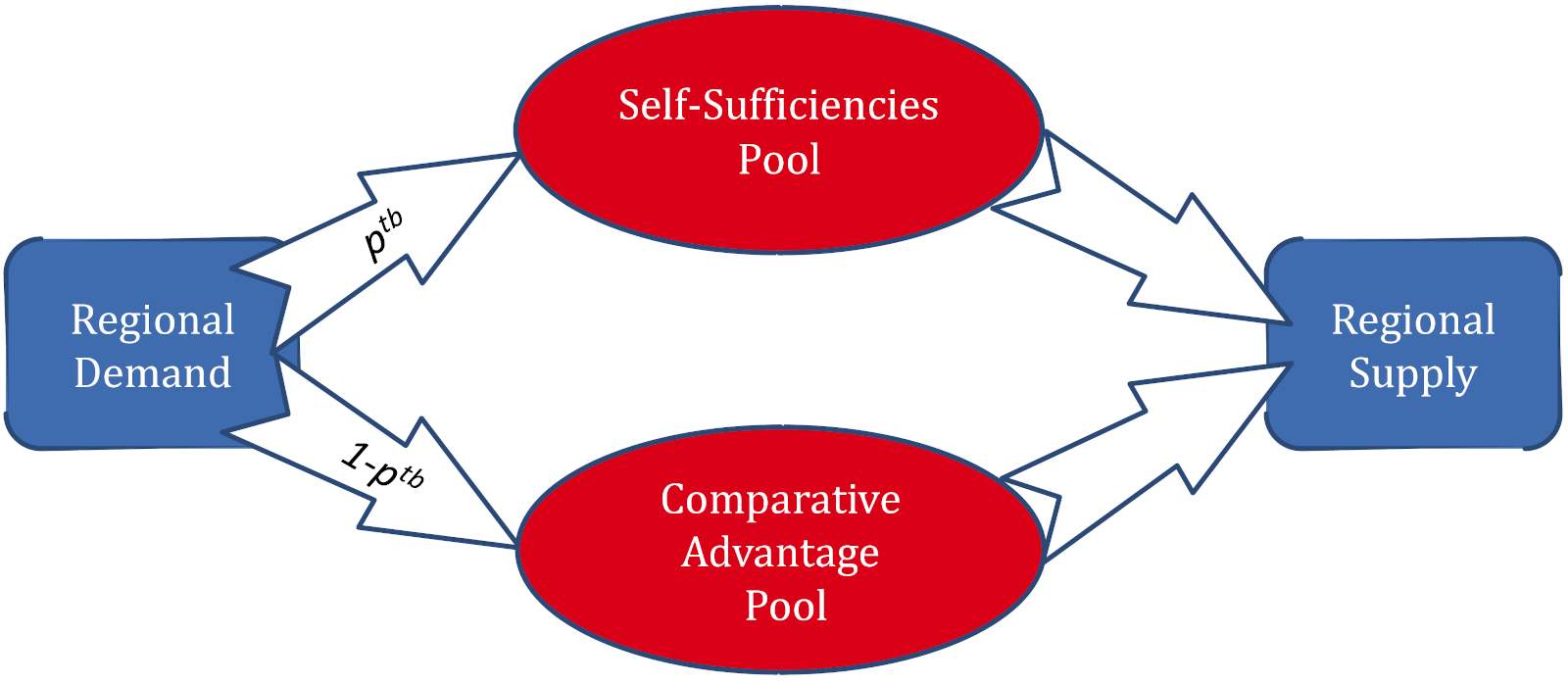
Effectively, this factor splits the global demand into two pools: The
ptb share of demand goes into a pool for which the origin
of products is fixed by the self-sufficiency ratios and export shares.
This “self-sufficiency” pool thus implies minimum production levels in
superregions, which are enforced by the lower bound of the production
band. The remaining part of the demand can be allocated more freely
based on comparative advantage in production of different superregions,
though still being constrained by the upper bounds of the production
band.
The superregional self-sufficiency ratios f21_self_suff
define how much of the demand of each superregion h for
each traded good k_trade is met by domestic production.
Self-sufficiency ratios smaller than one indicate that the superregion
imports from the world market, while self-sufficiencies greater than one
indicate that the superregion produces for export. The superregional
export shares f21_exp_shr distribute the total excess
demand of the importing superregions to the exporting superregions.
Trade costs are the sum of trade margins (international transport costs) and trade tariffs.
In the comparative advantage pool, the main constraint is that the global supply is larger or equal to demand. This means that production can be freely allocated globally based on comparative advantages.
\[\begin{multline*} \sum_{i2 }vm\_prod\_reg(i2,k\_trade) \geq \sum_{i2} vm\_supply(i2,k\_trade) + \sum_{ct}f21\_trade\_balanceflow(ct,k\_trade) \end{multline*}\]
For non-tradable commodites, the superregional supply should be larger or equal to the superregional demand.
\[\begin{multline*} \sum_{supreg(h2,i2)}vm\_prod\_reg(i2,k\_notrade) \geq \sum_{supreg(h2,i2)} vm\_supply(i2,k\_notrade) \end{multline*}\]
The following equations define the production band. The share of
demand that has to be fulfilled through the self-sufficiency pool is
determined by a trade balance reduction factor for each commodity
i21_trade_bal_reduction(ct,k_trade) (Schmitz et al. 2012). If the trade
balance reduction equals 1, all demand enters the self-sufficiency pool.
If it equals 0, all demand enters the comparative advantage pool. Note
that m21_baseline_production is a macro defined in
core/macros.gms. Lower bound for production.
\[\begin{multline*} \sum_{supreg(h2,i2)}vm\_prod\_reg(i2,k\_trade) \geq m21\_baseline\_production\left(vm\_supply, v21\_excess\_prod, f21\_self\_suff\right) \cdot \sum_{ct}i21\_trade\_bal\_reduction(ct,k\_trade) - v21\_import\_for\_feasibility(h2,k\_trade) \end{multline*}\]
Upper bound for production.
\[\begin{multline*} \sum_{supreg(h2,i2)}vm\_prod\_reg(i2,k\_trade) \leq \frac{ m21\_baseline\_production\left(vm\_supply, v21\_excess\_prod, f21\_self\_suff\right) }{ \sum_{ct}i21\_trade\_bal\_reduction(ct,k\_trade)} \end{multline*}\]
The global excess demand of each tradable good
v21_excess_demad equals to the sum over all the imports of
importing superregions.
\[\begin{multline*} v21\_excess\_dem(k\_trade) \geq \sum_{h2}\left( \sum_{supreg(h2,i2)}vm\_supply(i2,k\_trade) \cdot \left(1 - \sum_{ct}f21\_self\_suff(ct,h2,k\_trade)\right) \$\left(\sum_{ct}f21\_self\_suff(ct,h2,k\_trade) < 1\right)\right) + \sum_{ct}f21\_trade\_balanceflow(ct,k\_trade) + \sum_{h2} v21\_import\_for\_feasibility(h2,k\_trade) \end{multline*}\]
Distributing the global excess demand to exporting superregions is based on export shares (Schmitz et al. 2012). Export shares are derived from FAO data (see Schmitz et al. (2012) for details). They are 0 for importing superregions.
\[\begin{multline*} v21\_excess\_prod(h2,k\_trade) = v21\_excess\_dem(k\_trade) \cdot \sum_{ct}i21\_exp\_shr(ct,h2,k\_trade) \end{multline*}\]
\[\begin{multline*} \sum_{supreg(h2,i2)}vm\_cost\_trade\_tariff(i2) \geq \sum_{k\_trade}\left( i21\_trade\_tariff(h2,k\_trade) \cdot \sum\left(supreg(h2,i2), vm\_prod\_reg(i2,k\_trade) - vm\_supply(i2,k\_trade)\right)\right) \end{multline*}\]
\[\begin{multline*} \sum_{supreg(h2,i2)}vm\_cost\_trade\_margin(i2) \geq \sum_{k\_trade}\left( i21\_trade\_margin(h2,k\_trade) \cdot \sum\left(supreg(h2,i2), vm\_prod\_reg(i2,k\_trade) - vm\_supply(i2,k\_trade)\right)\right) \end{multline*}\]
\[\begin{multline*} \sum_{supreg(h2,i2)}vm\_cost\_trade\_feasibility(i2) \geq \sum_{k\_trade}\left( v21\_import\_for\_feasibility(h2,k\_trade) \cdot s21\_cost\_import\right) \end{multline*}\]
Trade liberalization i.e. shift from self-sufficiency fixed pool to free pool begins with sm_fix_SSP2 to keep values matching historical data until then.
Limitations This realization depends on predetermined self-sufficiency rates and export shares, which leads to a relative fixed trade pattern.
This realization implements bilateral trade between world regions based on historically observed import supply ratios. The import supply ratio expresses the share of an importing region’s domestic supply that is sourced from a specific exporting region, i.e. x% of region i’s supply of product k must be imported from exporter j. These ratios are derived from FAOSTAT bilateral trade data and held forward from the last observed historical period.
Trade volumes are constrained by upper and lower bounds around the historical import supply ratio, with a relaxation window defined by the observed standard deviation of these ratios over recent history. Formally, for each exporter-importer-product combination:
supply(im,k) * [ratio(ex,im,k) * scenarioFactor - libFactor * stddev(ex,im,k)] <= trade(ex,im,k) <= supply(im,k) * [ratio(ex,im,k) * scenarioFactor + libFactor * stddev(ex,im,k)]
The scenarioFactor
(i21_import_supply_scenario) allows scaling the historical
ratios up or down over time (e.g. to simulate trade liberalization or
protectionism). The libFactor
(i21_stddev_lib_factor) widens or narrows the flexibility
window around the historical pattern.
Within these bounds, the optimizer allocates trade to minimize total costs, which include bilateral transport margins and bilateral tariffs. Margins represent freight and insurance costs between specific region pairs. Tariffs are specific duty rates (USD per tDM) that can be faded out over a configurable time horizon. Margins and tariffs are applied to the traded volume and assigned to the exporting region.
Scenario-specific adjustments to individual bilateral ratios can be
applied via f21_trade_scenario_adjustments (controlled by
c21_trade_scenario), selecting a named geopolitical
scenario (USAex, CHAdom, EURex) or “off”. When a scenario is selected,
hardcoded additive perturbations are written into the zero-initialized
adjustment table and applied to the historical ratios from sm_fix_SSP2
onward, enabling targeted policy experiments such as reducing a
country’s import dependence on a specific trading partner.
The standard deviation bounds open from the simulation year (sm_fix_SSP2) onwards, with the level opening based on historically observed standard deviations, with the first 5 year time step at the max std observed over the all 5 years moving windows of the historical period for the exporter-importer and product combination. 10 years into the simulation period, the std dev window opens to the max std dev observed over all 10 year moving windows over the historical period, and the same happens at 15 years, after which the window remains fixed at the maximum observed historical standard deviation, allowing the flexibility window to evolve over time.
Non-tradable commodities (fodder, pasture, residues, bioenergy crops) are constrained to be produced within the super-region where they are consumed. A regional production constraint including trade flows ensures that world production covers total world supply plus any balance flows.
Regional production must cover regional supply plus bilateral trade flows plus historic balance flows. Regional material balance: production within a super-region must cover domestic supply minus imports plus exports, adjusted by historic balance flows as described above. Regional Imports are the sum of trade flowing into region i from all exporters; exports are the sum of trade flowing out of region i to all importers as recorded in trade matrix v21_trade. Two balance flows are included to ensure that historic values are consistent with FAO mass balance data. First balanceflow is a regional balanceflow, as in the FAO mass balance data to which we calibrate, regional production and supply including net-trade are not equal. This can potentially stem from storage (not included in our accounting), or other inventory and data reporting discrepancies. Furthermore, the bilateral trade import supply ratios to which we calibrate are based on the FAO bilateral trade matrix, which was scaled to match FAO mass balance imports. However, it thus can’t be scaled to also match FAO mass balance exports, and therefore we need to calibrate total regional exports to match non-bilateral exports. This amount may also stem from time spent in transit (also stored in transit), along with data discrepancies in FAOSTAT. Both balance flows are faeded to 0 by 2030, only ensuring historic consistency with FAO mass balance data.
\[\begin{multline*} \sum_{supreg\left(h2, i2\right)}\left( vm\_prod\_reg\left(i2, k\_trade\right)\right) \geq \sum_{supreg(h2,i2)}\left( vm\_supply\left(i2, k\_trade\right) - \sum_{i\_ex}\left( v21\_trade\left(i\_ex, i2, k\_trade\right)\right) + \sum_{i\_im}\left( v21\_trade\left(i2, i\_im, k\_trade\right)\right) + \sum_{ct}\left( f21\_trade\_export\_balanceflow\left(ct, i2, k\_trade\right)\right) + \sum_{ct}\left( f21\_trade\_regional\_balanceflow\left(ct, i2, k\_trade\right)\right)\right) \end{multline*}\]
For non-tradable commodities, the regional supply should be larger or equal to the regional demand.
\[\begin{multline*} \sum_{supreg(h2,i2)}vm\_prod\_reg(i2,k\_notrade) \geq \sum_{supreg(h2,i2)} vm\_supply(i2,k\_notrade) \end{multline*}\]
Lower bound on bilateral trade: each exporter-importer flow must be
at least the importer’s supply multiplied by the historical import
supply ratio (optionally scaled by
i21_import_supply_scenario), minus a flexibility window
defined by the historical standard deviation times the liberalization
factor. A larger i21_stddev_lib_factor widens the window
and allows trade to deviate further below the historical pattern.
\[\begin{multline*} v21\_trade(i\_ex,i\_im,k\_trade) \geq vm\_supply(i\_im,k\_trade) \cdot \sum_{ct}\left( i21\_import\_supply\_historical(i\_ex,i\_im,ct,k\_trade) \cdot i21\_import\_supply\_scenario(ct) - i21\_stddev\_lib\_factor(ct) \cdot i21\_trade\_bilat\_stddev(ct,i\_ex,i\_im,k\_trade)\right) \end{multline*}\]
Upper bound on bilateral trade: each exporter-importer flow must not
exceed the importer’s supply multiplied by the historical import supply
ratio, plus the flexibility window (standard deviation times
liberalization factor). Together with q21_trade_lower,
these bounds create a corridor around the historical bilateral trade
pattern within which the optimizer can adjust flows to minimize total
costs.
\[\begin{multline*} v21\_trade(i\_ex,i\_im,k\_trade) \leq vm\_supply(i\_im,k\_trade) \cdot \sum_{ct}\left( i21\_import\_supply\_historical(i\_ex,i\_im,ct,k\_trade) + i21\_stddev\_lib\_factor(ct) \cdot i21\_trade\_bilat\_stddev(ct,i\_ex,i\_im,k\_trade)\right) \end{multline*}\]
Tariff costs for each exporting region are the sum over all bilateral flows of the traded volume times the bilateral specific duty tariff rate (USD/tDM). Tariffs are assigned to the exporting region.
\[\begin{multline*} v21\_cost\_tariff\_reg(i2,k\_trade) = \sum_{ct,i\_im}\left( v21\_trade(i2,i\_im,k\_trade) \cdot i21\_trade\_tariff(ct,i2,i\_im,k\_trade)\right) \end{multline*}\]
Transport margin costs (freight and insurance) for each exporting region are the sum of bilateral margin rates times traded volumes across all importers. Margins are defined at the bilateral region-pair level, reflecting region-to-region trade costs’.
\[\begin{multline*} v21\_cost\_margin\_reg(i2,k\_trade) \geq \sum_{i\_im}\left( i21\_trade\_margin(i2,i\_im,k\_trade) \cdot v21\_trade(i2,i\_im,k\_trade)\right) \end{multline*}\]
Tariff costs per region aggregated over all tradable commodities. This variable enters the global objective function.
\[\begin{multline*} vm\_cost\_trade\_tariff(i2) = \sum_{k\_trade} v21\_cost\_tariff\_reg(i2,k\_trade) \end{multline*}\]
Transport margin costs per region aggregated over all tradable commodities. This variable enters the global objective function.
\[\begin{multline*} vm\_cost\_trade\_margin(i2) = \sum_{k\_trade} v21\_cost\_margin\_reg(i2,k\_trade) \end{multline*}\]
Limitations Trade patterns are anchored to historically observed bilateral import supply ratios, so structural shifts in trade partnerships beyond the scenario adjustments are not endogenously modeled. The standard deviation window provides some flexibility but does not capture potential new trade corridors with no historical precedent. Bilateral margins and tariffs are static inputs (with optional tariff fadeout) and do not respond endogenously to price changes. The realization operates at the MAgPIE world-region level rather than country level.
| Description | Unit | A | B | C | |
|---|---|---|---|---|---|
| f21_dom_supply (t_all, h, kall) |
Superregional domestic supply | \(10^6 tDM/yr\) | x | ||
| f21_import_supply_historical (i_ex, i_im, t_all, k_trade) |
Share of importer domestic supply sourced from each exporter derived from FAOSTAT | \(1\) | x | ||
| f21_self_suff (t_all, h, kall) |
Superregional self-sufficiency rates | \(1\) | x | x | |
| f21_trade_balanceflow (t_all, kall) |
Domestic balance flows | \(10^6 tDM/yr\) | x | ||
| f21_trade_balance (t_all, h, kall) |
trade balance of positive exports and negative imports | \(10^6 tDM/yr\) | x | ||
| f21_trade_bal_reduction (t_all, trade_groups21, trade_regime21) |
Share of inelastic trade pool | \(1\) | x | ||
| f21_trade_bilat_stddev (i_ex, i_im, k_trade, trade_stddev21) |
Standard deviation of import supply ratios over rolling windows of 5 10 and 15 years | \(1\) | x | ||
| f21_trade_export_balanceflow (t_all, i, k_trade) |
Balanceflow to match historic inconsistencies between trade matrix exports and FAO massbalance | \(10^6 tDM/yr\) | x | ||
| f21_trade_margin (h, kall) |
Costs of freight and insurance | \(USD_{17MER}/tDM\) | x | x | x |
| f21_trade_regional_balanceflow (t_all, i, kall) |
Balanceflow to match historic inconsistencies between supply and demand | \(10^6 tDM/yr\) | x | ||
| f21_trade_scenario_adjustments (i_ex, i_im, t_all, k_trade) |
Exogenous additive adjustments to bilateral import supply ratios for policy scenarios | \(1\) | x | ||
| f21_trade_tariff (h, kall) |
Specific duty tariffs | \(USD_{17MER}/tDM\) | x | x | x |
| i21_exp_glo (t_all, k_trade) |
Total global exports | \(tDM\) | x | ||
| i21_exports (t_all, h, k_trade) |
Total exports | \(tDM\) | x | ||
| i21_exp_shr (t_all, h, k_trade) |
Trade export shr | \(1\) | x | ||
| i21_import_supply_historical (i_ex, i_im, t_all, k_trade) |
Share of importer domestic supply sourced from each exporter - historical and projected | \(1\) | x | ||
| i21_import_supply_scenario (t_all) |
Time-varying scalar on import supply ratios for scenario experiments | \(1\) | x | ||
| i21_stddev_lib_factor (t_all) |
Time-varying scalar on the flexibility window width | \(1\) | x | ||
| i21_trade_bal_reduction (t_all, k_trade) |
Trade balance reduction | \(1\) | x | ||
| i21_trade_bilat_stddev (t_all, i_ex, i_im, k_trade) |
Standard deviation of historical import supply ratios used as flexibility window | \(1\) | x | ||
| i21_trade_margin (h, k_trade) |
Trade margins | \(USD_{17MER}/tDM\) | x | x | x |
| i21_trade_tariff (h, k_trade) |
Trade tariffs | \(USD_{17MER}/tDM\) | x | x | x |
| q21_costs_margins (i, k_trade) |
Bilateral transport margin costs assigned to exporting region | \(10^6 USD_{17MER}/yr\) | x | ||
| q21_costs_tariffs (i, k_trade) |
Bilateral tariff costs assigned to exporting region | \(10^6 USD_{17MER}/yr\) | x | ||
| q21_cost_trade_feasibility (h) |
Superregional feasibility penalty costs | \(10^6 USD_{17MER}/yr\) | x | ||
| q21_cost_trade_margin (h) |
Superregional margin costs | \(10^6 USD_{17MER}/yr\) | x | x | x |
| q21_cost_trade_tariff (h) |
Superregional tariff costs | \(10^6 USD_{17MER}/yr\) | x | x | x |
| q21_excess_dem (k_trade) |
Global excess demand | \(10^6 tDM/yr\) | x | ||
| q21_excess_supply (h, k_trade) |
Superregional excess production | \(10^6 tDM/yr\) | x | ||
| q21_notrade (h, kall) |
Superregional production constraint of non-tradable commodities | \(10^6 tDM/yr\) | x | x | x |
| q21_trade_glo (k_trade) |
Global production constraint | \(10^6 tDM/yr\) | x | ||
| q21_trade_lower (i_ex, i_im, k_trade) |
Lower bound on bilateral trade from historical import supply ratio minus flexibility | \(10^6 tDM/yr\) | x | ||
| q21_trade_reg (h, k_trade) |
Superregional trade balances i.e. minimum self-sufficiency ratio | \(1\) | x | x | |
| q21_trade_reg_up (h, k_trade) |
Superregional trade balances i.e. maximum self-sufficiency ratio | \(1\) | x | ||
| q21_trade_upper (i_ex, i_im, k_trade) |
Upper bound on bilateral trade from historical import supply ratio plus flexibility | \(10^6 tDM/yr\) | x | ||
| s21_cost_import | Cost for additional imports to maintain feasibility | \(USD_{17MER}/tDM\) | x | x | |
| s21_import_supply_scenario | Multiplicative factor on the line | x | |||
| s21_import_supply_scenario_targetyear | Target year for fade in | x | |||
| s21_min_trade_margin_forestry | Minimum trade margin for forestry products | \(USD_{17MER}/tDM\) | x | x | x |
| s21_stddev_lib_factor | Multiplicative factor on the window | x | |||
| s21_trade_scenario_adjustments | Switch to apply scenario adjustments to import supply | \(0=off 1=on\) | x | ||
| s21_trade_tariff | Trade tariff switch (1=on 0=off) | \(1\) | x | x | x |
| s21_trade_tariff_factor | Target multiplier for trade tariff fade | \(1=no change 0=fade to zero\) | x | ||
| s21_trade_tariff_startyear | Year to start fading trade tariffs towards target multiplier | x | |||
| s21_trade_tariff_targetyear | Year to finish fading trade tariffs towards target multiplier | x | |||
| v21_cost_margin_reg (i, k_trade) |
Regional transport margin costs summed over all bilateral partners | \(10^6 USD_{17MER}/yr\) | x | ||
| v21_cost_tariff_reg (i, k_trade) |
Regional tariff costs summed over all bilateral partners | \(10^6 USD_{17MER}/yr\) | x | ||
| v21_excess_dem (k_trade) |
Global excess demand | \(10^6 tDM/yr\) | x | ||
| v21_excess_prod (h, k_trade) |
Superregional excess production | \(10^6 tDM/yr\) | x | ||
| v21_import_for_feasibility (h, k_trade) |
Additional imports to maintain feasibility | \(10^6 tDM/yr\) | x | ||
| v21_trade (i_ex, i_im, k_trade) |
Bilateral trade flow from exporter to importer | \(10^6 tDM/yr\) | x |
| description | |
|---|---|
| ct(t) | Current time period |
| h | all superregional economic regions |
| h2(h) | Superregional (dynamic set) |
| i | all economic regions |
| i2(i) | World regions (dynamic set) |
| kall | All products in the sectoral version |
| k_hardtrade21(k_trade) | Products where trade should be limited |
| k_import21(k_trade) | Commodities that can have additional imports to maintain feasibility |
| k_notrade(kall) | Production activities of non-tradable commodites |
| k_trade(kall) | Production activities of tradable commodities |
| supreg(h, i) | mapping of superregions to its regions |
| t_all(t_ext) | 5-year time periods |
| trade_groups21 | Trade groups |
| trade_regime21 | Trade scenarios |
| trade_stddev21 | Standard deviation of observed bilateral trade |
| tstart21(t_all) | Historic time steps |
| t(t_all) | Simulated time periods |
| type | GAMS variable attribute used for the output |
Xiaoxi Wang, Anne Biewald, Christoph Schmitz, Markus Bonsch
09_drivers, 11_costs, 16_demand, 17_production